Machine Learning Module in OSCR

OSCR Machine Learning in Python

Linear Regression Module

© Kaixin Wang, Fall 2019

A PDF version of the tutorial can be accessed here

Module/Package import

import numpy as np # numpy module for linear algebra
import pandas as pd # pandas module for data manipulation
import matplotlib.pyplot as plt # module for plotting
import seaborn as sns # another module for plotting

import warnings # to handle warning messages
warnings.filterwarnings('ignore')

from sklearn.linear_model import LinearRegression # package for linear model
import statsmodels.api as sm # another package for linear model
import statsmodels.formula.api as smf
import scipy as sp

from sklearn.model_selection import train_test_split # split data into training and testing sets

Dataset import

The dataset that we will be using is the meuse dataset.

As described by the author of the data: “This data set gives locations and topsoil heavy metal concentrations, along with a number of soil and landscape variables at the observation locations, collected in a flood plain of the river Meuse, near the village of Stein (NL). Heavy metal concentrations are from composite samples of an area of approximately 15 m $\times$ 15 m.”

soil = pd.read_csv("soil.csv")  # data import
soil.head() # check if read in correctly

	x	y	cadmium	copper	lead	zinc	elev	dist	om	ffreq	soil	lime	landuse	dist.m
0	181072	333611	11.7	85	299	1022	7.909	0.001358	13.6	1	1	1	Ah	50
1	181025	333558	8.6	81	277	1141	6.983	0.012224	14.0	1	1	1	Ah	30
2	181165	333537	6.5	68	199	640	7.800	0.103029	13.0	1	1	1	Ah	150
3	181298	333484	2.6	81	116	257	7.655	0.190094	8.0	1	2	0	Ga	270
4	181307	333330	2.8	48	117	269	7.480	0.277090	8.7	1	2	0	Ah	380

soil.shape # rows x columns

(155, 14)

print(soil.describe())

                   x              y     cadmium      copper        lead  \
count     155.000000     155.000000  155.000000  155.000000  155.000000   
mean   180004.600000  331634.935484    3.245806   40.316129  153.361290   
std       746.039775    1047.746801    3.523746   23.680436  111.320054   
min    178605.000000  329714.000000    0.200000   14.000000   37.000000   
25%    179371.000000  330762.000000    0.800000   23.000000   72.500000   
50%    179991.000000  331633.000000    2.100000   31.000000  123.000000   
75%    180629.500000  332463.000000    3.850000   49.500000  207.000000   
max    181390.000000  333611.000000   18.100000  128.000000  654.000000   

              zinc        elev        dist          om       ffreq  \
count   155.000000  155.000000  155.000000  153.000000  155.000000   
mean    469.716129    8.165394    0.240017    7.478431    1.606452   
std     367.073788    1.058657    0.197702    3.432966    0.734111   
min     113.000000    5.180000    0.000000    1.000000    1.000000   
25%     198.000000    7.546000    0.075687    5.300000    1.000000   
50%     326.000000    8.180000    0.211843    6.900000    1.000000   
75%     674.500000    8.955000    0.364067    9.000000    2.000000   
max    1839.000000   10.520000    0.880389   17.000000    3.000000   

             soil        lime       dist.m  
count  155.000000  155.000000   155.000000  
mean     1.451613    0.283871   290.322581  
std      0.636483    0.452336   226.799927  
min      1.000000    0.000000    10.000000  
25%      1.000000    0.000000    80.000000  
50%      1.000000    0.000000   270.000000  
75%      2.000000    1.000000   450.000000  
max      3.000000    1.000000  1000.000000  

index = pd.isnull(soil).any(axis = 1)
soil = soil[-index]
soil = soil.reset_index(drop = True)

soil.shape

(152, 14)

n = soil.shape[1]

Exploratory Data Analysis (EDA)

Let suppose that the variable we are intereted in is the variable lead.

1. Correlation Heatmap

plt.figure(figsize = (10, 8))
sns.heatmap(soil.corr(), annot = True, square = True, linewidths = 0.1)
plt.ylim(n-1, 0)
plt.xlim(0, n-1)
plt.title("Pearson Correlation Heatmap between variables")
plt.show()
soil.corr()["lead"].sort_values()

png

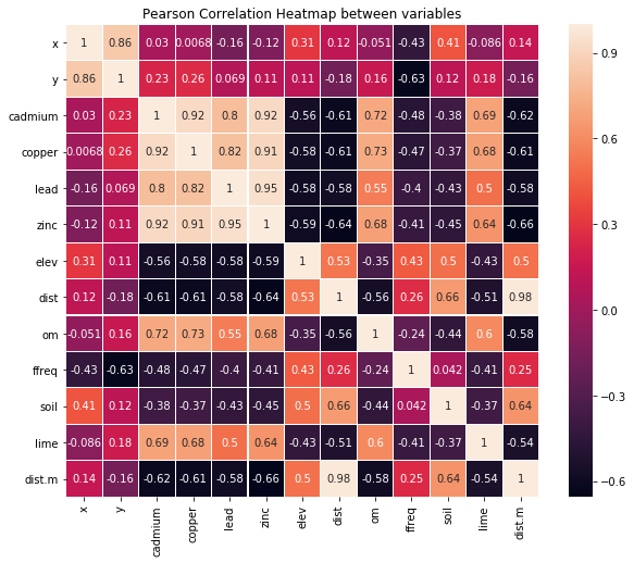
elev      -0.584323
dist.m    -0.584204
dist      -0.576577
soil      -0.430423
ffreq     -0.399238
x         -0.158104
y          0.069192
lime       0.501632
om         0.547836
cadmium    0.800898
copper     0.817000
zinc       0.954303
lead       1.000000
Name: lead, dtype: float64

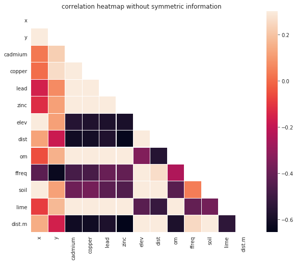
plt.figure(figsize = (10, 8))
corr = soil.corr()
mask = np.zeros_like(corr)
mask[np.triu_indices_from(mask)] = True
with sns.axes_style("white"):
    sns.heatmap(corr, mask = mask, linewidths = 0.1, vmax = .3, square = True)
plt.ylim(n-1, 0)
plt.xlim(0, n-1)
plt.title("correlation heatmap without symmetric information")
plt.show()

png

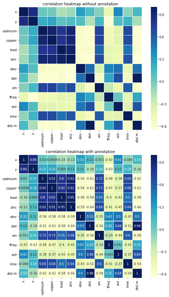
fig, axs = plt.subplots(figsize = (8, 12))
plt.subplots_adjust(left=0, bottom=0, right=1, top=1, wspace=0, hspace=0.2)
plt.subplot(2, 1, 1)
# correlation heatmap without annotation
sns.heatmap(soil.corr(), linewidths = 0.1, square = True, cmap = "YlGnBu")
plt.ylim(n-1, 0)
plt.xlim(0, n-1)
plt.title("correlation heatmap without annotation")
plt.subplot(2, 1, 2)
# correlation heatmap with annotation
sns.heatmap(soil.corr(), linewidths = 0.1, square = True, annot = True, cmap = "YlGnBu")
plt.ylim(n-1, 0)
plt.xlim(0, n-1)
plt.title("correlation heatmap with annotation")
plt.show()

png

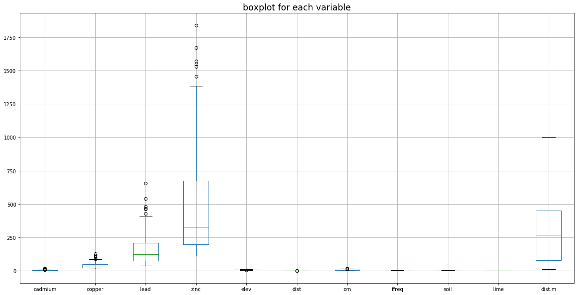
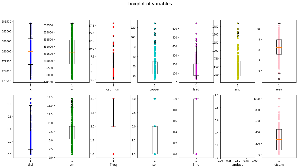
 2. Boxplots

plt.figure(figsize = (20, 10))
soil.iloc[:, 2:].boxplot()
# soil.iloc[:, 2:].plot(kind = "box")  # 2nd method
plt.title("boxplot for each variable", fontsize = "xx-large")
plt.show()

png

fig, axs = plt.subplots(2, int(n/2), figsize = (20, 10))
colors = ['b', 'g', 'r', 'c', 'm', 'y', 'pink']  # to set color

for i, var in enumerate(soil.columns.values):
    if var == "landuse":
        axs[1, i-int(n/2)].set_xlabel(var, fontsize = 'large')
        continue
    if i < int(n/2):
        axs[0, i].boxplot(soil[var])
        axs[0, i].set_xlabel(var, fontsize = 'large')
        axs[0, i].scatter(x = np.tile(1, soil.shape[0]), y = soil[var], color = colors[i])
    else:
        axs[1, i-int(n/2)].boxplot(soil[var])
        axs[1, i-int(n/2)].set_xlabel(var, fontsize = 'large')
        axs[1, i-int(n/2)].scatter(x = np.tile(1, soil.shape[0]), y = soil[var], 
                                   color = colors[i-int(n/2)])
        
plt.suptitle("boxplot of variables", fontsize = 'xx-large')
plt.show()

png

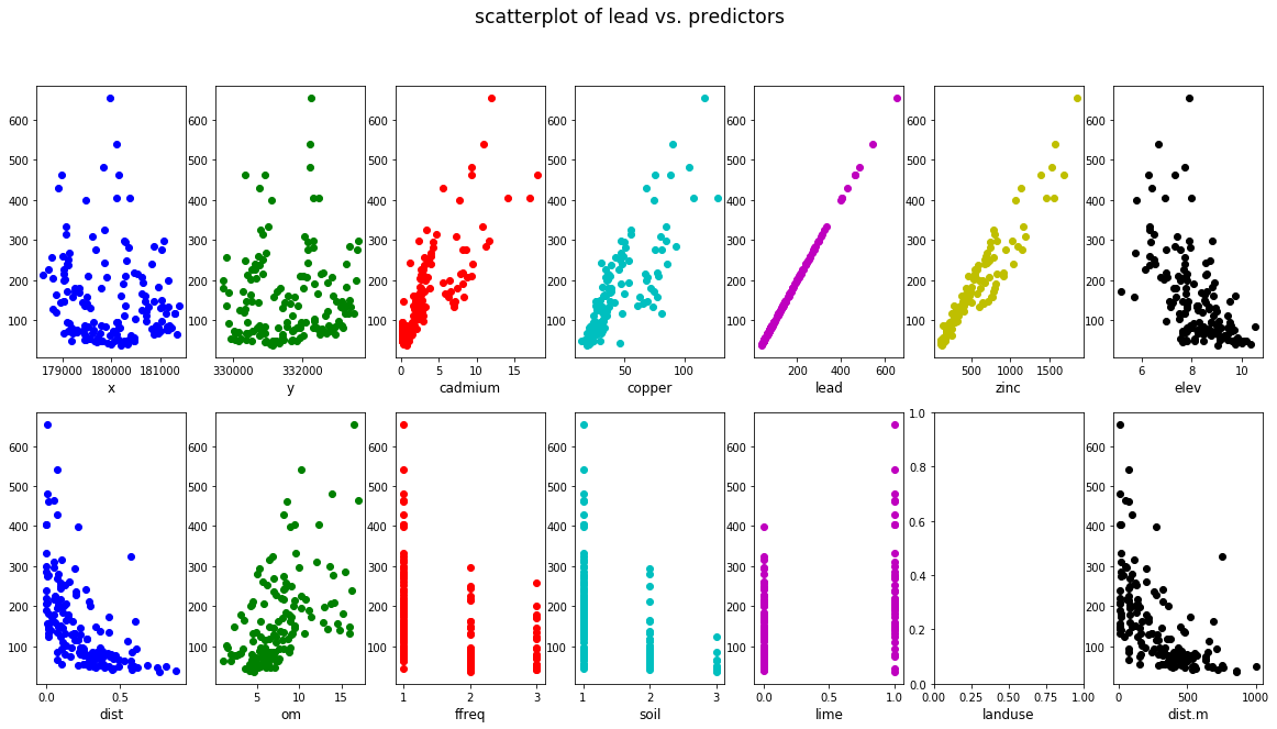
3. scatterplots

fig, axs = plt.subplots(2, int(n/2), figsize = (20, 10))
colors = ['b', 'g', 'r', 'c', 'm', 'y', 'k']  # to set color

for i, var in enumerate(soil.columns.values):
    if var == "landuse":
        axs[1, i-int(n/2)].set_xlabel(var, fontsize = 'large')
        continue
    if i < int(n/2):
        axs[0, i].scatter(soil[var], soil["lead"], color = colors[i])
        axs[0, i].set_xlabel(var, fontsize = 'large')
    else:
        axs[1, i-int(n/2)].scatter(soil[var], soil["lead"], color = colors[i-int(n/2)])
        axs[1, i-int(n/2)].set_xlabel(var, fontsize = 'large')
        
plt.suptitle("scatterplot of lead vs. predictors", fontsize = 'xx-large')
plt.show()

png

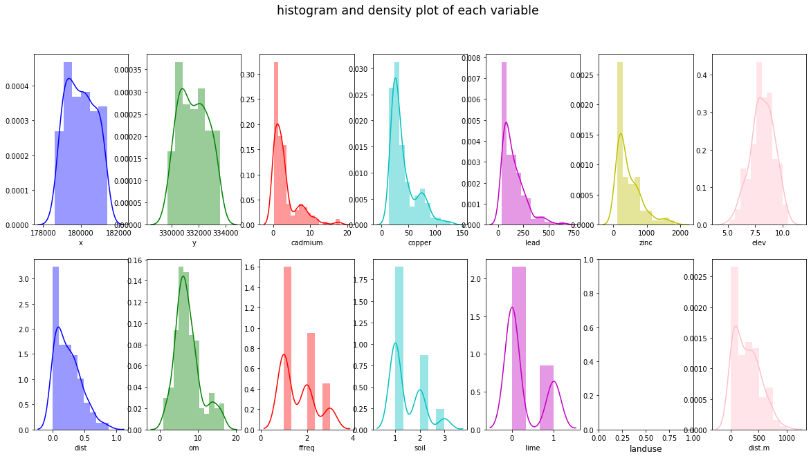
4. histograms and density plots

fig, axs = plt.subplots(2, int(n/2), figsize = (20, 10))
colors = ['b', 'g', 'r', 'c', 'm', 'y', 'pink']  # to set color

for i, var in enumerate(soil.columns.values):
    if var == "landuse":
        axs[1, i-int(n/2)].set_xlabel(var, fontsize = 'large')
        continue
    if i < int(n/2):
        sns.distplot(soil[var], color = colors[i], ax = axs[0, i])
    else:
        sns.distplot(soil[var], color = colors[i-int(n/2)], ax = axs[1, i-int(n/2)])
        
plt.suptitle("histogram and density plot of each variable", fontsize = 'xx-large')
plt.show()

png

Variable Selection and Modeling

Based on the scatterplot of lead vs. predictors:

cadmium, copper, zinc and om seem to have strong positive correlation with lead
elev, dist and dist.m seem to have strong negative correlation with lead
categorical variable lime seems to be a good indicator predictor variable

Therefore, we now build a linear model using 6 predictors: cadmium, copper, zinc, elev, dist and lime.

# variables = ["cadmium", "copper", "zinc", "elev", "dist", "dist.m", "lime"]
variables = ["cadmium", "copper", "zinc", "elev", "dist",  "lime"]

x = soil[variables]
y = soil["lead"]

Modeling - building a linear model

split the dataset into training and testing set

X_train, X_test, y_train, y_test = train_test_split(x, y, test_size = 0.33, random_state = 42)

build a linear model using sklearn package

model = LinearRegression().fit(X_train, y_train)

# R^2 on training set
R2_train = model.score(X_train, y_train)
R2_train

0.9483947080189404

# R^2 on testing set
R2_test = model.score(X_test, y_test)
R2_test

0.964901551899052

# value of intercepts
for var, coef in zip(variables, model.coef_):
    print(var, coef)

cadmium -13.391990002100986
copper 0.05365863276389149
zinc 0.42346584485869393
elev -3.2531127698493183
dist 14.509965024252311
lime -23.514058405476963

build a linear model using statsmodel package

df_train = pd.concat([X_train, y_train], axis = 1) # build a dataframe for training set

fullModel = smf.ols("lead ~ cadmium + copper + zinc + elev + C(lime)", data = df_train)

fullModel = fullModel.fit()
print(fullModel.summary())

                            OLS Regression Results                            
==============================================================================
Dep. Variable:                   lead   R-squared:                       0.948
Model:                            OLS   Adj. R-squared:                  0.945
Method:                 Least Squares   F-statistic:                     346.6
Date:                Tue, 12 Nov 2019   Prob (F-statistic):           2.35e-59
Time:                        08:17:24   Log-Likelihood:                -467.76
No. Observations:                 101   AIC:                             947.5
Df Residuals:                      95   BIC:                             963.2
Df Model:                           5                                         
Covariance Type:            nonrobust                                         
================================================================================
                   coef    std err          t      P>|t|      [0.025      0.975]
--------------------------------------------------------------------------------
Intercept       23.8739     27.200      0.878      0.382     -30.126      77.874
C(lime)[T.1]   -24.7610      7.775     -3.185      0.002     -40.196      -9.326
cadmium        -13.2322      2.240     -5.908      0.000     -17.679      -8.785
copper           0.0522      0.278      0.187      0.852      -0.500       0.605
zinc             0.4188      0.020     20.756      0.000       0.379       0.459
elev            -2.4719      2.895     -0.854      0.395      -8.220       3.276
==============================================================================
Omnibus:                        2.077   Durbin-Watson:                   1.947
Prob(Omnibus):                  0.354   Jarque-Bera (JB):                1.494
Skew:                          -0.246   Prob(JB):                        0.474
Kurtosis:                       3.336   Cond. No.                     6.42e+03
==============================================================================

Warnings:
[1] Standard Errors assume that the covariance matrix of the errors is correctly specified.
[2] The condition number is large, 6.42e+03. This might indicate that there are
strong multicollinearity or other numerical problems.

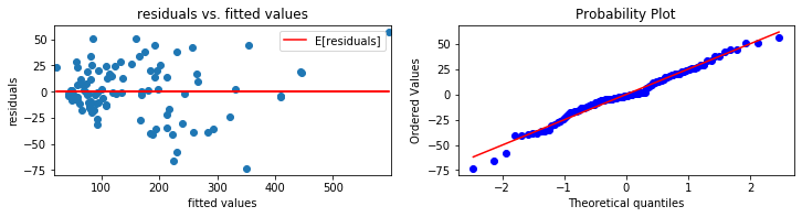
diagnostics plots

# diagnosticsPlots function definition
def diagnosticsPlots(predictions, truevalues):
    '''
    This function will plot the following two diagonistics plots:
    1. residuals vs. fitted values plot (plot on the left)
    2. qqplot of the residuals (plot on the right)
    
    parameters required:
    - predictions: predicted values using the linear regression model
    - truevalues:  true values of the response variable
    
    required modules/packages:
    - matplotlib.pyplot (plt)
    - scipy (sp)
    
    Author: Kaixin Wang
    Created: October 2019
    '''
    residuals = truevalues - predictions
    fig, axs = plt.subplots(figsize = (12, 2.5))
    plt.subplot(1, 2, 1)
    # residuals vs. fitted values
    plt.scatter(predictions, residuals)
    plt.plot(predictions, np.tile(np.mean(residuals), residuals.shape[0]), "r-")
    plt.xlim([np.min(predictions) - 2.5, np.max(predictions) + 2.5])
    plt.title("residuals vs. fitted values")
    plt.ylabel("residuals")
    plt.xlabel("fitted values")
    plt.legend(["E[residuals]"])
    print("Average of residuals: ", np.mean(residuals))
    # qqplot
    plot = plt.subplot(1, 2, 2)
    sp.stats.probplot(residuals, plot = plot, fit = True)
    plt.show()

pred_val = fullModel.fittedvalues.copy()
true_val = y_train.copy()
diagnosticsPlots(pred_val, true_val)

Average of residuals:  2.583420825998257e-12

png

training and testing Root-Mean-Square Error (RMSE)

The root-mean-square error of a prediction is calcuated as the following:

$\text{RMSE} = \frac{\sqrt{\sum_{i=1}^n (y_i - \hat {y_i}) ^ 2}}{n}$

where $y_i$ is the true value of the response, $\hat {y_i}$ is the fitted value of the response, n is the size of the input

def RMSETable(train_y, train_fitted, train_size, train_R2, test_y, test_fitted, test_size, test_R2):
    '''
    This function creates a function that returns a dataframe in the following format:
    -------------------------------------------------
                     RMSE     R-squared    size 
    training set  train_RMSE  train_R2    n_training
    testing set   test_RMSE   tesint_R2   n_testing
    -------------------------------------------------
    
    parameters required:
    - train_y: true values of the response in the training set
    - train_fitted: fitted values of the response in the training set
    - train_size: size of the training set
    - train_R2: R-squared on the training set
    - test_y: true values of the response in the testing set
    - test_fitted: fitted values of the response in the testing set
    - test_size: size of the testing size
    - test_R2: R-squared on the testing set
    
    Author: Kaixin Wang
    Created: October 2019
    '''
    train_RMSE = np.sqrt(sum(np.power(train_y - train_fitted, 2))) / train_size
    test_RMSE  = np.sqrt(sum(np.power(test_y  - test_fitted, 2))) / test_size
    train = [train_RMSE, train_size, train_R2]
    test  = [test_RMSE,  test_size,  test_R2]
    return pd.DataFrame([train, test], index = ["training set", "testing set"], columns = ["RMSE", "R-squared", "size"])

table1 = RMSETable(y_train.values, model.predict(X_train), R2_train, len(y_train), 
                   y_test.values, model.predict(X_test), R2_test, len(y_test))
print(table1)

                    RMSE  R-squared  size
training set  262.286912   0.948395   101
testing set   159.247070   0.964902    51

Model selection

Since we are using 5 predictor variables for 152 entries, we can consider using fewer predictors to improve the $R_{adj}^2$, where is a version of $R^2$ that penalizes model complexity.

Selecting fewer predictor will also help with preventing overfitting.

Therefore, observing that zinc, copper and cadmium have relatively stronger correlation with lead, we now build a model using only these three predictors.

using sklearn linear regression module

variables = ["cadmium", "lime", "zinc"]
x = soil[variables]
y = soil["lead"]
X_train, X_test, y_train, y_test = train_test_split(x, y, test_size = 0.33, random_state = 42)

model2 = LinearRegression().fit(X_train, y_train)
# R^2 on training set
R2_train = model2.score(X_train, y_train)
print("Training set R-squared", R2_train)
# R^2 on testing set
R2_test = model2.score(X_test, y_test)
print("Testing set R-squared", R2_test)

Training set R-squared 0.9475953381623881
Testing set R-squared 0.9609072316593821

# value of intercepts
for var, coef in zip(variables, model2.coef_):
    print(var, coef)

cadmium -13.093360663968943
lime -23.487105420923648
zinc 0.4236873112817108

using statsmodel ordinary linear regrssion module

df_train = pd.concat([X_train, y_train], axis = 1) # build a dataframe for training set
reducedModel = smf.ols("lead ~ cadmium + C(lime) + zinc", data = df_train)
reducedModel = reducedModel.fit()
print(reducedModel.summary())

                            OLS Regression Results                            
==============================================================================
Dep. Variable:                   lead   R-squared:                       0.948
Model:                            OLS   Adj. R-squared:                  0.946
Method:                 Least Squares   F-statistic:                     584.7
Date:                Tue, 12 Nov 2019   Prob (F-statistic):           5.98e-62
Time:                        08:17:24   Log-Likelihood:                -468.19
No. Observations:                 101   AIC:                             944.4
Df Residuals:                      97   BIC:                             954.8
Df Model:                           3                                         
Covariance Type:            nonrobust                                         
================================================================================
                   coef    std err          t      P>|t|      [0.025      0.975]
--------------------------------------------------------------------------------
Intercept        2.6976      4.614      0.585      0.560      -6.461      11.856
C(lime)[T.1]   -23.4871      7.569     -3.103      0.003     -38.509      -8.465
cadmium        -13.0934      1.986     -6.593      0.000     -17.035      -9.152
zinc             0.4237      0.019     22.540      0.000       0.386       0.461
==============================================================================
Omnibus:                        0.749   Durbin-Watson:                   1.968
Prob(Omnibus):                  0.688   Jarque-Bera (JB):                0.395
Skew:                          -0.131   Prob(JB):                        0.821
Kurtosis:                       3.160   Cond. No.                     1.79e+03
==============================================================================

Warnings:
[1] Standard Errors assume that the covariance matrix of the errors is correctly specified.
[2] The condition number is large, 1.79e+03. This might indicate that there are
strong multicollinearity or other numerical problems.

diagnostics plots

pred_val = reducedModel.fittedvalues.copy()
true_val = y_train.copy()
diagnosticsPlots(pred_val, true_val)

Average of residuals:  3.392313932510102e-13

png

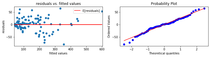
table2 = RMSETable(y_train.values, model2.predict(X_train), R2_train, len(y_train), 
                   y_test.values, model2.predict(X_test), R2_test, len(y_test))
print(table2)

                    RMSE  R-squared  size
training set  264.533494   0.947595   101
testing set   168.763005   0.960907    51

model evaluation and comparison

model with 5 predictors (full model)

print(table1)

                    RMSE  R-squared  size
training set  262.286912   0.948395   101
testing set   159.247070   0.964902    51

model with 3 predictors (reduced model)

print(table2)

                    RMSE  R-squared  size
training set  264.533494   0.947595   101
testing set   168.763005   0.960907    51

table = sm.stats.anova_lm(reducedModel, fullModel)
table

	df_resid	ssr	df_diff	ss_diff	F	Pr(>F)
0	97.0	62835.802512	0.0	NaN	NaN	NaN
1	95.0	62309.421080	2.0	526.381432	0.401273	0.670596

Comparing the tables obtained above:

The full model with 6 predictors has lower test RMSE and higher $R^2$ value than the reduced model with 3 predictors
However, a higher $R^2$ doesn’t mean that we favor the full model, since $R^2$ will always increase as the number of predictors used increases. Instead, we will take a look at $R^2_{adj}$, the adjusted $R^2$, which is calculated as

$R^2_{adj} = 1 - (1 - R^2) \frac{n - 1}{n - p - 1}$

where $n$ is the sample size and $p$ is the number of predictors used in the model.

Since $R_{adj}^2$ of the full model is 0.945, while the $R_{adj}^2$ of the reduced model is 0.946, which is an improvement, we observe that the reduced model has a lower model complexity while maintaining a good prediction performance.

Summary of the module

By building two linear regression models using 6 and 3 predictors respectively, we observe that predictor variables cadmium, copper and zinc have very strong positive correlation with the response variable lead. In addition, we also observed that by adding three more predictors, dist, elev and lime, the $R^2_{adj}$ didn’t get much improvement comparing to the model with only 3 predictors.

Therefore, the final model that we decided to adopt is the reduced model with 3 predictors:

$\text{Lead} \sim \text{Cadmium} + \text{lime} + \text{Zinc}$

Reference:

Dataset: meuse dataset

P.A. Burrough, R.A. McDonnell, 1998. Principles of Geographical Information Systems. Oxford University Press.
Stichting voor Bodemkartering (STIBOKA), 1970. Bodemkaart van Nederland : Blad 59 Peer, Blad 60 West en 60 Oost Sittard: schaal 1 : 50 000. Wageningen, STIBOKA.

To access this dataset in R:

install.packages("sp")
library(sp)
data(meuse)