
CPI Prediction Project
CPI Prediction Project
Group memebers: Kaixin Wang, Qin Hu, Ruby Zhang, and Emily Suan
Time: Statistics 131 - Spring 2019
1. Objective:
Predict CPI (customer price index) of countries using predictors relevant to economic growth.
2. Introduction:
Datasets:
- GDP_and_GDP_Per_Capita.csv (1)
- Expenditure_on_Health.csv (2)
- Production_Trade_and_Supply_of_Energy.csv (3)
- Internet_Usage.csv (4)
- Public_Expenditure_on_Education.csv (5)
- Tourist_Visitors_Arrival_and_Expenditure.csv (6)
- GDP_on_R&D.csv (7)
- Exchange_Rates.csv (8)
- Consumer_Price_Index.csv (9)
Variables from datasets:
- response: CPI (9)
- predictors:
- GDP (1)
- expenditure on health (2)
- energy usage (3)
- Internet usage (4)
- expenditure on education (5)
- expenditure on tourism (6)
- expenditure on science & technology (7)
- exchange rate (8)
Datasets sources:
United Nations: http://data.un.org/
- National accounts (1)
- GDP and GDP per capita
- Nutrition and health (2)
- Health expenditure
- Energy (3)
- Energy production, trade and consumption
- Communication (4)
- Internet usage
- Education (5)
- Public expenditure on education
- Science and technology (7)
- Human resources in R & D
- Finance (8)
- Exchange rates
- Price and production indices (9)
- Consumer price indices
3. Data Clean-up:
import numpy as np
import pandas as pd
import matplotlib.pyplot as plt
import seaborn as sns
# handling warning messages:
import warnings
warnings.filterwarnings('ignore')
CPI = pd.read_csv("Consumer_Price_Index.csv", encoding ="ISO-8859-1")
CPI.Series.unique()      # to extra certain rows
CPI = CPI.loc[CPI.Series == 'Consumer price index: General']
countries = CPI.Country.unique()
CPI.head()
CPI.describe()
| ID | Year | Value | |
|---|---|---|---|
| count | 1243.000000 | 1243.00000 | 1243.000000 |
| mean | 422.092518 | 2010.87852 | 113.465245 |
| std | 248.315099 | 6.85628 | 142.542578 |
| min | 4.000000 | 1995.00000 | 0.000000 |
| 25% | 212.000000 | 2010.00000 | 98.300000 |
| 50% | 418.000000 | 2014.00000 | 106.900000 |
| 75% | 634.000000 | 2016.00000 | 120.300000 |
| max | 894.000000 | 2017.00000 | 4583.700000 |
- The Consumer Price Index (CPI) is a measure of the average change over time in the prices paid by urban consumers for a market basket of consumer goods and services.
- It can be calculated as updated cost divided by base period cost times 100.
- In this project, we only consider the general market.
The annual percentage change in a CPI is used as a measure of inflation. Generally, if increase rate of CPI in one year is larger than 3%, the country can be considered as having an inflation.
- The data set provides CPI of 1995 to 2017 for each country.
CPI of year 2010 is set as an index base of 100. For example, Afghanistan at year 2014 had a value of 133.1, this can be interpreted as that there was 33.1% increase in inflation since 2010.
- The origin of data is United Nations Statistics Division (UNSD), New York, Monthly Bulletin of Statistics (MBS), last accessed May 2018.
health = pd.read_csv("Expenditure_on_Health.csv", encoding ="ISO-8859-1")
health = health.loc[health.Series == 'Current health expenditure (% of GDP)']
health.head()
health.Value.describe()
count    1129.000000
mean        6.406112
std         2.915264
min         0.800000
25%         4.400000
50%         5.900000
75%         8.000000
max        26.300000
Name: Value, dtype: float64
- The value is the percentage of GDP that each country expends on health.
The data set provides values of 2000 to 2015 for each country.
The average percentage is 6.4, the median is 5.9, and the 75th percentile is 8.0. So we can see that Afghanistan relatively has more percentage that spends on health than average.
- The origin of data is World Health Organization (WHO), Geneva, WHO Global Health Expenditure database, last accessed March 2018. The estimates are in line with the 2011 System of Health Accounts (SHA).
GDP = pd.read_csv("GDP_and_GDP_Per_Capita.csv", encoding ="ISO-8859-1")
gdp = GDP.loc[GDP.Series == "GDP per capita (US dollars)"]
gdp.Value.describe()
count      1451.000000
mean      12586.084080
std       20869.037211
min          79.000000
25%        1171.000000
50%        3932.000000
75%       14755.000000
max      168003.000000
Name: Value, dtype: float64
- The gross domestic product (GDP) is a monetary measure of the market value of all the final goods and services produced in a period of time.
- The GDP per capita divides the country’s GDP by its total population.
- The data set provides GDP of 1985 to 2017 for each country.
The unit is in millions of US dollars at current and constant 2010 prices.
The average GDP per capita is 12586.1, the median is 3932.0, and the 75th percentile is 14755.0. So we can see that Afghanistan has a relatively low GDP per capita.
- The origin of data is United Nations Statistics Division, New York, National Accounts Statistics: Analysis of Main Aggregates (AMA) database, last accessed February 2018.
energy = pd.read_csv("Production_Trade_and_Supply_of_Energy.csv", encoding ="ISO-8859-1" )
energy = energy.loc[energy.Series == "Primary energy production (petajoules)"]
energy.Value.describe()
count      1651.000000
mean       2294.987886
std        8565.910899
min           0.000000
25%           8.000000
50%         132.000000
75%         971.500000
max      101498.000000
Name: Value, dtype: float64
- Primary energy sources include fossil fuels (petroleum, natural gas, and coal), nuclear energy, and renewable sources of energy.
- The data set provides data of 1990 to 2016 for each country.
The unit of energy is in petajoule. 1 Petajoule equals to a quadrillion joules. 10^15 joules.
The average value is 2295.0, the median is 132.0, and the 75th percentile is 971.5. So we can see that Afghanistan has a relatively low primary energy production.
- The origin of data is United Nations Statistics Division, New York, Energy Statistics Yearbook 2016, last accessed January 2019.
internet = pd.read_csv("Internet_Usage.csv", encoding ="ISO-8859-1" )
internet.Value.describe()
count    1506.000000
mean       38.198340
std        30.419562
min         0.000000
25%         9.100000
50%        33.250000
75%        65.000000
max        99.000000
Name: Value, dtype: float64
- The value shows the percentage of individuals using the internet.
The data set provides percentage of 2000 to 2017 for each country.
The average value is 38.2, the median is 33.3, and the 75th percentile is 65.0. So we can see that Afghanistan has a relatively low percentage of internet usage.
- The origin of data is International Telecommunication Union (ITU), Geneva, the ITU database, last accessed January 2019.
education = pd.read_csv("Public_Expenditure_on_Education.csv", encoding ="ISO-8859-1" )
education = education.loc[education.Series == "Public expenditure on education (% of government expenditure)"]
education.Value.describe()
count    577.000000
mean      15.015251
std        5.388521
min        0.800000
25%       11.100000
50%       14.400000
75%       18.200000
max       44.800000
Name: Value, dtype: float64
- The value measures the percentage of public expenditure on education over goverment expenditure.
The years range from 2000 to 2018.
The average value is 15.0, the median is 14.4, and the 75th percentile is 18.2. So we can see that Albania has a relatively low percentage of educational expenditure.
- The origin of data is United Nations Educational, Scientific and Cultural Organization (UNESCO), Montreal, the UNESCO Institute for Statistics (UIS) statistics database, last accessed March 2019.
tourism = pd.read_csv("Tourist_Visitors_Arrival_and_Expenditure.csv", encoding ="ISO-8859-1" )
tourism = tourism.loc[tourism.Series == "Tourism expenditure (millions of US dollars)"]
tourism.Value.describe()
count      1079.000000
mean       6025.848007
std       17792.255719
min           0.000000
25%         171.500000
50%         828.000000
75%        4508.000000
max      251361.000000
Name: Value, dtype: float64
- Tourism expenditure refers to the total consumption expenditure made by a visitor, or on behalf of a visitor for goods and services during his/her trip and stay at the destination place (country). It also includes payments in advance or after the trip for services received during the trip.
The data set provides data of 1995 to 2017 for each country.
The average value is 6025.8, the median is 828.0, and the 75th percentile is 4508.0. So we can see that Afghanistan has a relatively low tourism expenditure.
- The origin of data is World Tourism Organization (UNWTO), Madrid, the UNWTO Statistics Database, last accessed January 2019.
technology = pd.read_csv("GDP_on_R&D.csv", encoding ="ISO-8859-1" )
tech = technology.loc[technology.Series == 'Gross domestic expenditure on R & D: as a percentage of GDP (%)']
tech.Value.describe()
count    431.000000
mean       0.852668
std        0.937531
min        0.000000
25%        0.200000
50%        0.500000
75%        1.200000
max        4.300000
Name: Value, dtype: float64
- The gross domestic spending on research and development (R&D) is defined as the total expenditure on R&D as a percentage of its GDP (in USD). It carried out by all resident companies, research institutes, university and government laboratories, etc., in a country. It is considered an indicator of the country’s degree of R&D intensity and is a commonly used summary statistic for international comparisons.
The years range from 2000 to 2016.
The average value is 0.85, the median is 0.50, and the 75th percentile is 1.20. So we can see that Albania has a relatively low expenditure on R&D.
- The origin of data is United Nations Educational, Scientific and Cultural Organization (UNESCO), Montreal, the UNESCO Institute for Statistics (UIS) statistics database, last accessed September 2018.
rates = pd.read_csv("Exchange_Rates.csv", encoding ="ISO-8859-1" )
rates = rates.loc[rates.Series == "Exchange rates: period average (national currency per US dollar)"]
rates.Value.describe()
count     1687.000000
mean       450.674155
std       2221.031597
min          0.000000
25%          1.200000
50%          6.000000
75%         90.100000
max      33226.300000
Name: Value, dtype: float64
- In finance, an exchange rate is the rate at which one currency will be exchanged for another. It is also regarded as the value of one country’s currency in relation to another currency.
- The value is the exchange rate of each country’s currency to USD in a specific year.
The data set provides data of 1985 to 2017 for each country.
An exchange rate appreciation causes a slower growth of real GDP because of a fall in net exports (reduced injection) and a rise in the demand for imports (an increased leakage in the circular flow). Thus, a higher exchange rate can have a negative multiplier effect on the economy.
The average value is 450.7, the median is 6.0, and the 75th percentile is 90.1. So we can see that Afghanistan has a relatively low exchange rate.
- The origin of data is International Monetary Fund (IMF), Washington, D.C., the database on International Financial Statistics supplemented by operational rates of exchange for United Nations programmes, last accessed June 2018.
gdp.pivot(index = "Year", columns = "Country", values = "Value").head()
| Country | Afghanistan | Albania | Algeria | Andorra | Angola | Anguilla | Antigua and Barbuda | Argentina | Armenia | Aruba | ... | United States of America | Uruguay | Uzbekistan | Vanuatu | Venezuela (Boliv. Rep. of) | Viet Nam | Yemen | Zambia | Zanzibar | Zimbabwe |
|---|---|---|---|---|---|---|---|---|---|---|---|---|---|---|---|---|---|---|---|---|---|
| Year | |||||||||||||||||||||
| 1985 | 282.0 | 783.0 | 2564.0 | 9837.0 | 859.0 | 4072.0 | 3508.0 | 3144.0 | NaN | 6108.0 | ... | 18017.0 | 1735.0 | NaN | 1020.0 | 3425.0 | 79.0 | NaN | 399.0 | NaN | 872.0 |
| 1995 | 189.0 | 770.0 | 1452.0 | 23359.0 | 466.0 | 10583.0 | 7841.0 | 7993.0 | 426.0 | 16442.0 | ... | 28758.0 | 6609.0 | 589.0 | 1621.0 | 3375.0 | 276.0 | 387.0 | 417.0 | 235.0 | 846.0 |
| 2005 | 264.0 | 2615.0 | 3100.0 | 41281.0 | 1891.0 | 18129.0 | 11453.0 | 5125.0 | 1753.0 | 23303.0 | ... | 44173.0 | 5221.0 | 543.0 | 1886.0 | 5433.0 | 684.0 | 925.0 | 691.0 | 408.0 | 481.0 |
| 2010 | 558.0 | 4056.0 | 4463.0 | 39734.0 | 3586.0 | 19459.0 | 12175.0 | 10346.0 | 3432.0 | 23513.0 | ... | 48574.0 | 11938.0 | 1382.0 | 2966.0 | 13566.0 | 1310.0 | 1309.0 | 1463.0 | 587.0 | 720.0 |
| 2015 | 611.0 | 3895.0 | 4163.0 | 36040.0 | 4171.0 | 22622.0 | 13602.0 | 14853.0 | 3618.0 | 25796.0 | ... | 56948.0 | 15525.0 | 2160.0 | 2871.0 | 11054.0 | 2065.0 | 990.0 | 1319.0 | 795.0 | 1033.0 |
5 rows × 214 columns
# pivoting all datasets:
CPI = CPI.pivot(index = "Year", columns = "Country", values = "Value")
GDP = gdp.pivot(index = "Year", columns = "Country", values = "Value")
energy = energy.pivot(index = "Year", columns = "Country", values = "Value")
health = health.pivot(index = "Year", columns = "Country", values = "Value")
education = education.pivot(index = "Year", columns = "Country", values = "Value")
tech = tech.pivot(index = "Year", columns = "Country", values = "Value")
internet = internet.pivot(index = "Year", columns = "Country", values = "Value")
rates = rates.pivot(index = "Year", columns = "Country", values = "Value")
tourism = tourism.pivot(index = "Year", columns = "Country", values = "Value")
name = 'United States of America'
table1 = pd.DataFrame(CPI.loc[:, name])
table1 = pd.concat([table1, pd.DataFrame(GDP.loc[:, name]), pd.DataFrame(energy.loc[:, name]), pd.DataFrame(tech.loc[:, name]), pd.DataFrame(internet.loc[:, name]), pd.DataFrame(tourism.loc[:, name]), pd.DataFrame(health.loc[:, name])], keys = ["Energy", "Tech", "Education", "Internet", "Tourism", "Health"])
table1 = table1.swaplevel().unstack()
table1.fillna(method = "ffill", inplace = True)
table1.fillna(method = "bfill", inplace = True)
table1.head()
| United States of America | ||||||
|---|---|---|---|---|---|---|
| Energy | Tech | Education | Internet | Tourism | Health | |
| Year | ||||||
| 1985 | 69.9 | 18017.0 | 68588.0 | 2.5 | 43.1 | 93743.0 |
| 1990 | 69.9 | 18017.0 | 68588.0 | 2.5 | 43.1 | 93743.0 |
| 1995 | 69.9 | 28758.0 | 68963.0 | 2.5 | 43.1 | 93743.0 |
| 2000 | 69.9 | 28758.0 | 69339.0 | 2.5 | 43.1 | 93743.0 |
| 2001 | 69.9 | 28758.0 | 69339.0 | 2.5 | 43.1 | 93743.0 |
name = 'China'
table2 = pd.DataFrame(CPI.loc[:, name])
table2 = pd.concat([table2, pd.DataFrame(GDP.loc[:, name]), pd.DataFrame(energy.loc[:, name]), pd.DataFrame(tech.loc[:, name]), pd.DataFrame(rates.loc[:, name]), pd.DataFrame(internet.loc[:, name]), pd.DataFrame(tourism.loc[:, name]), pd.DataFrame(health.loc[:, name])], keys = ["Energy", "Tech", "Rates", "Internet", "Tourism", "Health"])
table2 = table2.swaplevel().unstack()
table2.fillna(method = "ffill", inplace = True)
table2.fillna(method = "bfill", inplace = True)
table2.head()
| China | ||||||
|---|---|---|---|---|---|---|
| Energy | Tech | Rates | Internet | Tourism | Health | |
| Year | ||||||
| 1985 | 100.0 | 289.0 | 32727.0 | 1.3 | 2.9 | 1.8 |
| 1990 | 100.0 | 289.0 | 32727.0 | 1.3 | 2.9 | 1.8 |
| 1995 | 100.0 | 592.0 | 39692.0 | 1.3 | 8.4 | 1.8 |
| 2000 | 100.0 | 592.0 | 40783.0 | 1.3 | 8.4 | 1.8 |
| 2001 | 100.0 | 592.0 | 40783.0 | 1.3 | 8.4 | 1.8 |
4. Exploratory Data Analysis:
# processing data:
rates["United States of America"] = 1.0   # rates for US is always 1
education["China"] = 0                    # no entries for education of China
CPI["China"].loc[CPI["China"].index == 2016] = CPI["China"].loc[CPI["China"].index == 2015].iloc[0] * CPI["China"].loc[CPI["China"].index == 2016].iloc[0] / 100
CPI["China"].loc[CPI["China"].index == 2017] = CPI["China"].loc[CPI["China"].index == 2015].iloc[0]  * CPI["China"].loc[CPI["China"].index == 2017].iloc[0] / 100
years = CPI.index
# since CPI = 100 for year 2010 (base year)
years = [1995, 2005, 2014, 2015, 2016, 2017]
# G7 countires: United States of America, Germany, France, Japan, Canada, United Kingdon and Italy
# BRICS countires: Brazil, Russian Federation, India, China and South Africa
G7 = ["United States of America", "Germany", "France", "Japan", "Canada", "United Kingdom", "Italy"]
BRICS = ["Brazil", "Russian Federation", "India", "China", "South Africa"]
df1 = pd.DataFrame()
for name in G7:
    table = pd.DataFrame(CPI.loc[years, name])
    table = pd.concat([table, pd.DataFrame(GDP.loc[years, name]), pd.DataFrame(energy.loc[years, name]), pd.DataFrame(tech.loc[years, name]), pd.DataFrame(education.loc[years, name]), pd.DataFrame(rates.loc[years, name]), pd.DataFrame(internet.loc[years, name]), pd.DataFrame(tourism.loc[years, name]), pd.DataFrame(health.loc[years, name])], keys = ["CPI", "GDP", "Energy", "Tech", "Education", "Rates", "Internet", "Tourism", "Health"])
    table = table.swaplevel().unstack()
    table.fillna(method = "ffill", inplace = True)
    table.fillna(method = "bfill", inplace = True)
    df1 = pd.concat([df1, table], axis = 1)

df2 = pd.DataFrame()
for name in BRICS:
    table = pd.DataFrame(CPI.loc[years, name])
    table = pd.concat([table, pd.DataFrame(GDP.loc[years, name]), pd.DataFrame(energy.loc[years, name]), pd.DataFrame(tech.loc[years, name]), pd.DataFrame(education.loc[years, name]), pd.DataFrame(rates.loc[years, name]), pd.DataFrame(internet.loc[years, name]), pd.DataFrame(tourism.loc[years, name]), pd.DataFrame(health.loc[years, name])], keys = ["CPI", "GDP", "Energy", "Tech", "Education", "Rates", "Internet", "Tourism", "Health"])
    table = table.swaplevel().unstack()
    table.fillna(method = "ffill", inplace = True)
    table.fillna(method = "bfill", inplace = True)
    df2 = pd.concat([df2, table], axis = 1)

df1.fillna(0, inplace = True)
df2.fillna(0, inplace = True)
plt.figure(figsize = (9, 5))
for i in range(7):
    plt.plot(df1.index, df1[G7[i]].CPI, label = G7[i])
    plt.legend()
    plt.title("CPI vs. year for G7 countries")
plt.show()
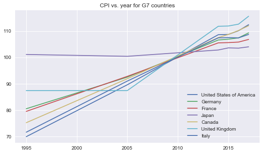
- For all G7 countries except Japan and United Kingdom, the CPI had continuously increased from 1995 to 2014, but the rate of increment had decreased from 2015 to 2017.
To achieve an economic growth, developed countries pursue a goal of 2% increment in CPI each year.
On the other hand, if the increase rate of CPI is low, the increase rate of prices would be low as well, thus customers would tend to delay purcahses and consumption, which in turn reduces overall economic activity and limits the economic growth.
CPI of Japan had maintained at around 102 in this time period because it was under depression. Japan had the highest CPI in 1995 but had the lowest CPI in 2017 compared to other G7 countries.
The line of CPI of United Kingdom is flat from year 1995 to 2005 because the CPI is missing in this time period. CPI of United Kingdom was the lowest in 2005, but it became the highest in 2017.
- Because CPI of year 2010 is set as an index base of 100, we can see in the plot, at year 2010, all countries had CPI of 100.
plt.figure(figsize = (9, 5))
for i in range(5):
plt.plot(df2.index, df2[BRICS[i]].CPI, label = BRICS[i])
plt.legend()
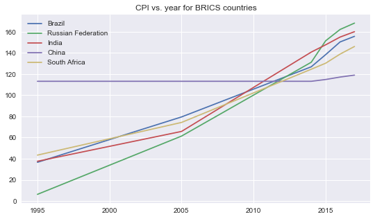
plt.title("CPI vs. year for BRICS countries")
plt.show()
# Final dataframe for modeling:
G7 = ["United States of America", "Germany", "France", "Japan", "Canada", "United Kingdom", "Italy"]
BRICS = ["Brazil", "Russian Federation", "India", "China", "South Africa"]
df1 = pd.DataFrame()
for name in G7:
    table = pd.DataFrame(CPI.stack().loc[list(years), name])
    table = pd.concat([table, pd.DataFrame(GDP.stack().loc[list(years), name]), pd.DataFrame(energy.stack().loc[list(years), name]), pd.DataFrame(tech.stack().loc[list(years), name]), pd.DataFrame(education.stack().loc[list(years), name]), pd.DataFrame(rates.stack().loc[list(years), name]), pd.DataFrame(internet.stack().loc[list(years), name]), pd.DataFrame(tourism.stack().loc[list(years), name]), pd.DataFrame(health.stack().loc[list(years), name])], keys = ["CPI", "GDP", "Energy", "Tech", "Education", "Rates", "Internet", "Tourism", "Health"], axis = 1)
    table.fillna(method = "ffill", inplace = True)
    table.fillna(method = "bfill", inplace = True)
    df1 = pd.concat([df1, table])

df2 = pd.DataFrame()
for name in BRICS:
    table = pd.DataFrame(CPI.stack().loc[list(years), name])
    table = pd.concat([table, pd.DataFrame(GDP.stack().loc[list(years), name]), pd.DataFrame(energy.stack().loc[list(years), name]), pd.DataFrame(tech.stack().loc[list(years), name]), pd.DataFrame(education.stack().loc[list(years), name]), pd.DataFrame(rates.stack().loc[list(years), name]), pd.DataFrame(internet.stack().loc[list(years), name]), pd.DataFrame(tourism.stack().loc[list(years), name]), pd.DataFrame(health.stack().loc[list(years), name])], keys = ["CPI", "GDP", "Energy", "Tech", "Education", "Rates", "Internet", "Tourism", "Health"], axis = 1)
    table.fillna(method = "ffill", inplace = True)
    table.fillna(method = "bfill", inplace = True)
    df2 = pd.concat([df2, table])

df1.fillna(0, inplace = True)
df2.fillna(0, inplace = True)

df1.columns = df1.columns.droplevel(1)
df1["Country"] = df1.index.get_level_values(1)
df1.index = df1.index.droplevel(1)
df2.columns = df2.columns.droplevel(1)
df2["Country"] = df2.index.get_level_values(1)
df2.index = df2.index.droplevel(1)
corr = df1.corr()
sns.heatmap(corr, xticklabels = corr.columns.values, yticklabels = corr.columns.values)
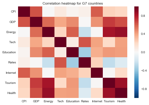
plt.title("Correlation heatmap for G7 countries")
plt.show()
corr
| CPI | GDP | Energy | Tech | Education | Rates | Internet | Tourism | Health | |
|---|---|---|---|---|---|---|---|---|---|
| CPI | 1.000000 | 0.635231 | 0.004209 | 0.094490 | 0.024644 | 0.057702 | 0.603672 | 0.226905 | 0.204881 |
| GDP | 0.635231 | 1.000000 | 0.566710 | 0.389412 | 0.472322 | 0.000052 | 0.448515 | 0.697273 | 0.643213 |
| Energy | 0.004209 | 0.566710 | 1.000000 | 0.218402 | 0.596894 | -0.228006 | 0.005587 | 0.833641 | 0.871232 |
| Tech | 0.094490 | 0.389412 | 0.218402 | 1.000000 | 0.079500 | 0.628720 | 0.403439 | 0.193145 | 0.412377 |
| Education | 0.024644 | 0.472322 | 0.596894 | 0.079500 | 1.000000 | -0.349489 | 0.366237 | 0.434638 | 0.416917 |
| Rates | 0.057702 | 0.000052 | -0.228006 | 0.628720 | -0.349489 | 1.000000 | 0.227365 | -0.245600 | -0.137512 |
| Internet | 0.603672 | 0.448515 | 0.005587 | 0.403439 | 0.366237 | 0.227365 | 1.000000 | 0.009633 | 0.194322 |
| Tourism | 0.226905 | 0.697273 | 0.833641 | 0.193145 | 0.434638 | -0.245600 | 0.009633 | 1.000000 | 0.856595 |
| Health | 0.204881 | 0.643213 | 0.871232 | 0.412377 | 0.416917 | -0.137512 | 0.194322 | 0.856595 | 1.000000 |
corr = df2.corr()
sns.heatmap(corr, xticklabels = corr.columns.values, yticklabels = corr.columns.values)
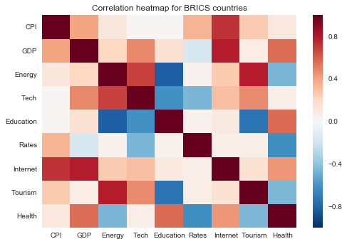
plt.title("Correlation heatmap for BRICS countries")
plt.show()
corr
| CPI | GDP | Energy | Tech | Education | Rates | Internet | Tourism | Health | |
|---|---|---|---|---|---|---|---|---|---|
| CPI | 1.000000 | 0.397548 | 0.114049 | 0.011822 | 0.009338 | 0.341825 | 0.719207 | 0.265609 | 0.106135 |
| GDP | 0.397548 | 1.000000 | 0.209489 | 0.483707 | 0.149363 | -0.169871 | 0.787094 | 0.073416 | 0.559502 |
| Energy | 0.114049 | 0.209489 | 1.000000 | 0.679992 | -0.825651 | 0.046559 | 0.259245 | 0.787208 | -0.458878 |
| Tech | 0.011822 | 0.483707 | 0.679992 | 1.000000 | -0.607607 | -0.456791 | 0.302228 | 0.474215 | 0.067872 |
| Education | 0.009338 | 0.149363 | -0.825651 | -0.607607 | 1.000000 | 0.045039 | 0.095796 | -0.736679 | 0.570032 |
| Rates | 0.341825 | -0.169871 | 0.046559 | -0.456791 | 0.045039 | 1.000000 | 0.059896 | 0.067193 | -0.620344 |
| Internet | 0.719207 | 0.787094 | 0.259245 | 0.302228 | 0.095796 | 0.059896 | 1.000000 | 0.154858 | 0.440551 |
| Tourism | 0.265609 | 0.073416 | 0.787208 | 0.474215 | -0.736679 | 0.067193 | 0.154858 | 1.000000 | -0.452931 |
| Health | 0.106135 | 0.559502 | -0.458878 | 0.067872 | 0.570032 | -0.620344 | 0.440551 | -0.452931 | 1.000000 |
# adding country_code variable:
# G7 countires: United States of America, Germany, France, Japan, Canada, United Kingdon and Italy
# BRICS countires: Brazil, Russian Federation, India, China and South Africa
code1 = {"United States of America" : 1, "Germany" : 2, "France" : 3, "Japan" : 4, "Canada" : 5,
         "United Kingdom" : 6, "Italy" : 7}
code2 = {"Brazil" : 8, "Russian Federation" : 9, "India" : 10, "China" : 11, "South Africa" : 12}
df1["Country_code"] = [code1[country] for country in df1.Country]
df2["Country_code"] = [code2[country] for country in df2.Country]
df1.head()
| CPI | GDP | Energy | Tech | Education | Rates | Internet | Tourism | Health | Country | Country_code | |
|---|---|---|---|---|---|---|---|---|---|---|---|
| Year | |||||||||||
| 1995 | 69.9 | 28758.0 | 68963.0 | 2.5 | 13.5 | 1.0 | 68.0 | 93743.0 | 14.5 | United States of America | 1 |
| 2005 | 89.6 | 44173.0 | 68124.0 | 2.5 | 13.5 | 1.0 | 68.0 | 122077.0 | 14.5 | United States of America | 1 |
| 2014 | 108.6 | 44173.0 | 83426.0 | 2.5 | 13.5 | 1.0 | 73.0 | 122077.0 | 16.5 | United States of America | 1 |
| 2015 | 108.7 | 56948.0 | 84051.0 | 2.5 | 13.5 | 1.0 | 74.6 | 249183.0 | 16.8 | United States of America | 1 |
| 2016 | 110.1 | 58064.0 | 79672.0 | 2.7 | 13.5 | 1.0 | 75.2 | 246172.0 | 16.8 | United States of America | 1 |
CPI.loc[years, G7].agg(["min","max"])
| United States of America | Germany | France | Japan | Canada | United Kingdom | Italy | |
|---|---|---|---|---|---|---|---|
| min | 69.9 | 80.5 | 79.5 | 100.4 | 75.2 | 87.4 | 71.6 |
| max | 112.4 | 109.3 | 106.8 | 104.0 | 112.0 | 115.6 | 108.7 |
CPI.loc[years, BRICS].agg(["min","max"])
| Brazil | Russian Federation | India | China | South Africa | |
|---|---|---|---|---|---|
| min | 36.6 | 6.3 | 37.6 | 113.2000 | 43.4 |
| max | 155.7 | 168.2 | 160.1 | 119.0364 | 146.1 |
# adding categorical label for response variable:
df1["CPI_Level"] = [4 if var > 150 else 3 if var > 120 else 2 if var > 80 else 1 for var in df1["CPI"]]
df2["CPI_Level"] = [4 if var > 150 else 3 if var > 120 else 2 if var > 80 else 1 for var in df2["CPI"]]
# reset the index of dataframes and create a column of years:
df1.reset_index(inplace = True)
df2.reset_index(inplace = True)
df2.head()
| Year | CPI | GDP | Energy | Tech | Education | Rates | Internet | Tourism | Health | Country | Country_code | CPI_Level | |
|---|---|---|---|---|---|---|---|---|---|---|---|---|---|
| 0 | 1995 | 36.6 | 4794.0 | 5038.0 | 1.0 | 11.3 | 0.9 | 21.0 | 1085.0 | 8.0 | Brazil | 8 | 1 |
| 1 | 2005 | 79.5 | 4770.0 | 8344.0 | 1.0 | 11.3 | 2.4 | 21.0 | 4168.0 | 8.0 | Brazil | 8 | 1 |
| 2 | 2014 | 126.9 | 4770.0 | 10965.0 | 1.0 | 15.7 | 2.4 | 54.6 | 4168.0 | 8.4 | Brazil | 8 | 3 |
| 3 | 2015 | 138.4 | 8750.0 | 11842.0 | 1.3 | 15.7 | 3.3 | 58.3 | 6254.0 | 8.9 | Brazil | 8 | 3 |
| 4 | 2016 | 150.4 | 8634.0 | 12183.0 | 1.3 | 15.7 | 3.5 | 60.9 | 6613.0 | 8.9 | Brazil | 8 | 4 |
# drop one entry in United Kingdom where CPI is missing:
print("Dimension before removing one missing obseration:", df1.shape)
df1.drop([31], inplace = True)
df1.reset_index(inplace = True)
df1.drop("index", axis = 1, inplace = True)
print("Dimension after removing one missing obseration:", df1.shape)
Dimension before removing one missing obseration: (42, 13)
Dimension after removing one missing obseration: (41, 13)
# remove two entries where CPI of China are missing:
print("Dimension before removing two missing obseration:", df2.shape)
df2.drop([18, 19], inplace = True)
df2.reset_index(inplace = True)
df2.drop("index", axis = 1, inplace = True)
print("Dimension before removing two missing obserations:", df2.shape)
Dimension before removing two missing obseration: (30, 13)
Dimension before removing two missing obserations: (28, 13)
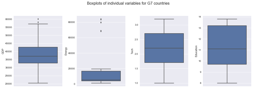
fig, (ax1, ax2, ax3, ax4) = plt.subplots(ncols=4,figsize=(20,8))
plt.suptitle("Boxplots of individual variables for G7 countries", fontsize=16,y=1.1,x=0.45)
plt.subplots_adjust(bottom = 0.5, right = 0.8, top = 1, wspace = 0.3)
sns.boxplot(y=df1['GDP'], ax=ax1)
sns.boxplot(y=df1['Energy'], ax=ax2)
sns.boxplot(y=df1['Tech'], ax=ax3)
sns.boxplot(y=df1['Education'], ax=ax4)
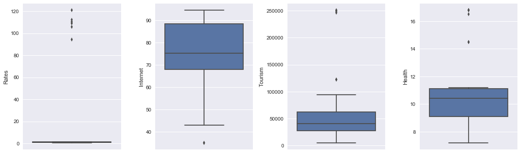
fig, (ax5, ax6, ax7, ax8) = plt.subplots(ncols=4,figsize=(20,8))
plt.subplots_adjust(bottom = 0.5, right = 0.8, top = 1, wspace = 0.35)
sns.boxplot(y=df1['Rates'], ax=ax5)
sns.boxplot(y=df1['Internet'], ax=ax6)
sns.boxplot(y=df1['Tourism'], ax=ax7)
sns.boxplot(y=df1['Health'], ax=ax8)
plt.show()
fig, (ax1, ax2, ax3, ax4) = plt.subplots(ncols=4,figsize=(20,8))
plt.suptitle("Boxplots of individual variables for BRICS countries", fontsize=16,y=1.1,x=0.45)
plt.subplots_adjust(bottom = 0.5, right = 0.8, top = 1, wspace = 0.3)
sns.boxplot(y=df2['GDP'], ax=ax1)
sns.boxplot(y=df2['Energy'], ax=ax2)
sns.boxplot(y=df2['Tech'], ax=ax3)
sns.boxplot(y=df2['Education'], ax=ax4)
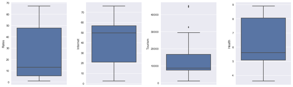
fig, (ax5, ax6, ax7, ax8) = plt.subplots(ncols=4,figsize=(20,8))
plt.subplots_adjust(bottom = 0.5, right = 0.8, top = 1, wspace = 0.35)
sns.boxplot(y=df2['Rates'], ax=ax5)
sns.boxplot(y=df2['Internet'], ax=ax6)
sns.boxplot(y=df2['Tourism'], ax=ax7)
sns.boxplot(y=df2['Health'], ax=ax8)
plt.show()
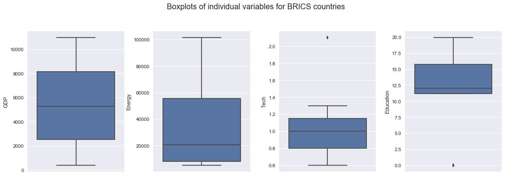
- GDP
- the median is around 5500 dollars.
- Energy
- the median is around 20000 petajoules.
- Tech
- the outliers are expenditure on tech of China in recent years, which exceeded other BRICS countries.
- the median of expenditure on tech is around 1% of GDP.
- Education
- the outliers are expenditure on education of China, which are missing values.
- the median of expenditure on education is around 12.5% of government expenditure.
- Rates
- the median of exchange rates is around 14.
- Internet
- the median of internet usage is around 50%.
- Tourism
- the outliers are tourism expenditure of China in recent years, which exceeded other BRICS countries.
- the median of tourism expenditure is around 9500 dollars.
- Health
- the median of health expenditure is around 5.6% of GDP.
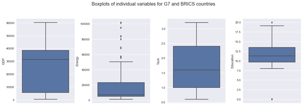
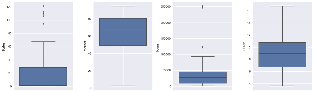
df = pd.concat([df1, df2])
fig, (ax1, ax2, ax3, ax4) = plt.subplots(ncols=4,figsize=(20,8))
plt.suptitle("Boxplots of individual variables for G7 and BRICS countries", fontsize=16,y=1.1,x=0.45)
plt.subplots_adjust(bottom = 0.5, right = 0.8, top = 1, wspace = 0.3)
sns.boxplot(y=df['GDP'], ax=ax1)
sns.boxplot(y=df['Energy'], ax=ax2)
sns.boxplot(y=df['Tech'], ax=ax3)
sns.boxplot(y=df['Education'], ax=ax4)
fig, (ax5, ax6, ax7, ax8) = plt.subplots(ncols=4,figsize=(20,8))
plt.subplots_adjust(bottom = 0.5, right = 0.8, top = 1, wspace = 0.35)
sns.boxplot(y=df['Rates'], ax=ax5)
sns.boxplot(y=df['Internet'], ax=ax6)
sns.boxplot(y=df['Tourism'], ax=ax7)
sns.boxplot(y=df['Health'], ax=ax8)
plt.show()
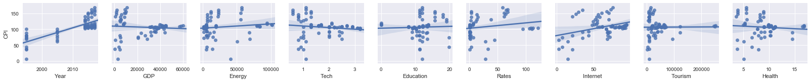
sns.pairplot(data = df1, y_vars = ['CPI'], x_vars = ['Year', 'GDP', 'Energy', 'Tech', 'Education', 'Rates', 'Internet', 'Tourism', 'Health'], kind = 'reg')
plt.show()
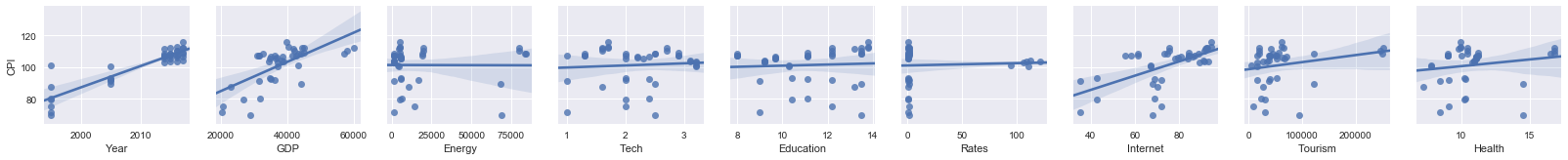
From this set of scatter plots, we observe that:
- CPI for G7 countries is positively related to Year, GDP, Rates, Internet and Tourism;
- the relation between CPI and variables such as Technology, Education, and Health are not as strong as other variables.
sns.pairplot(data = df2, y_vars = ['CPI'], x_vars = ['Year', 'GDP', 'Energy', 'Tech', 'Education', 'Rates', 'Internet', 'Tourism', 'Health'], kind = 'reg')
plt.show()
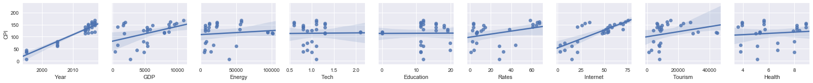
From this set of scatter plots for BRICS countries, we observe that:
- CPI is positively related to Year, GDP, Tech, Rates, Internet and Tourism;
- the relation between CPI and variables such as Energy, Education, and Health is not as strong.
sns.pairplot(data = df, y_vars = ['CPI'], x_vars = ['Year', 'GDP', 'Energy', 'Tech', 'Education', 'Rates', 'Internet', 'Tourism', 'Health'], kind = 'reg')
plt.show()
From this set of scatter plots for G7 and BRICS combined, we observe that:
- CPI is positively related to Year, Energy, Rates, and Internet;
- The relation between CPI and other variables such as Tech, Education, Tourism and Health is not as strong.
Summary for variables selected:
- CPI: Consumer price index (General)
- GDP: GDP per capita (US dollars)
- Energy: Primary energy production (petajoules)
- Tech: Gross domestic expenditure on R & D: as a percentage of GDP (%)
- Education: Public expenditure on education (% of government expenditure)
- Rates: Exchange rates: period average (national currency per US dollar)
- Internet: Percentage of individuals using the interne
- Tourism: Tourism expenditure (millions of US dollars)
- Health: Current health expenditure (% of GDP)
New created variables:
- Country: name of each country in G7 and BRICS
- Country_code: 1 - 7 for G7 countries, 8 - 12 for BRICS countries
- CPI_level: 1 - 4 based on CPI value:
- CPI > 150: high CPI (class 4)
- 120 < CPI <= 150: medium CPI (class 3)
- 80 <= CPI <= 120: stable CPI (class 2)
- CPI <= 80: low CPI (class 1)
5. Data Modeling:
Predictor variables:
- Year: categorical
- 6 levels: 1995, 2005, 2014, 2015, 2016, 2017
- Country_code:
- 7 levels for G7 (1 to 7)
- 5 levels for BRICS (8 to 12)
- GDP: numeric
- Energy: numeric
- Tech: numeric
- Education: numeric
- Rates: numeric
- Internet: numeric
- Tourism: numeric
- Health: numeric
- Group (used in multiple linear regression only): categorical
- 1 if the country is one of G7
- 2 if the country is one of BRICS
Response variable:
In part I: CPI_level
- categorical variable with 4 categories (1, 2, 3, and 4)
- CPI > 150: high CPI (class 4)
- 120 < CPI <= 150: medium CPI (class 3)
- 80 <= CPI <= 120: stable CPI (class 2)
- CPI <= 80: low CPI (class 1)
In part II: CPI
- numeric value of CPI
Structure:
Part I: predcition on range of CPI (categorical):
(1) G7 countries modeling:
- KNN classifier
- Naive Bayes classifier
(2) BRICS countires modeling:
- KNN classifier
- Naive Bayes classifier
(3) G7 and BRICS combined:
- KNN classifier
- Naive Bayes classifier
Part II: prediction on CPI (numeric):
Multiple regression models on:
- G7 countries
- BRICS countries
- G7 and BRICS combined
from sklearn.model_selection import train_test_split, cross_val_score
from sklearn.neighbors import KNeighborsClassifier
from sklearn.naive_bayes import GaussianNB
from sklearn.metrics import confusion_matrix
from sklearn.model_selection import GridSearchCV
from sklearn import linear_model, preprocessing, model_selection
# handling warning messages:
import warnings
warnings.filterwarnings('ignore')
Part I: predicting CPI as categorical variables:
Transform categorical variable using OneHotEncoder:
from sklearn.preprocessing import OneHotEncoder
encode = OneHotEncoder(sparse = False)
df1 = pd.concat([df1, pd.DataFrame(encode.fit_transform(df1[["Country_code"]]), columns = G7)], axis = 1)
df2 = pd.concat([df2, pd.DataFrame(encode.fit_transform(df2[["Country_code"]]), columns = BRICS)], axis = 1)
print(df1.columns)
print(df2.columns)
Index(['Year', 'CPI', 'GDP', 'Energy', 'Tech', 'Education', 'Rates',
       'Internet', 'Tourism', 'Health', 'Country', 'Country_code', 'CPI_Level',
       'United States of America', 'Germany', 'France', 'Japan', 'Canada',
       'United Kingdom', 'Italy'],
      dtype='object')
Index(['Year', 'CPI', 'GDP', 'Energy', 'Tech', 'Education', 'Rates',
       'Internet', 'Tourism', 'Health', 'Country', 'Country_code', 'CPI_Level',
       'Brazil', 'Russian Federation', 'India', 'China', 'South Africa'],
      dtype='object')
Cross Validation sets:
x1 = df1.iloc[:, [0,2,3,4,5,6,7,8,9,13,14,15,16,17,18,19]].astype(float)
y1 = df1.iloc[:, 12]
x2 = df2.iloc[:, [0,2,3,4,5,6,7,8,9,13,14,15,16,17]].astype(float)
y2 = df2.iloc[:, 12]

x1_train, x1_test, y1_train, y1_test = train_test_split(x1, y1, test_size = 0.2, random_state = 1, stratify = df1.Country_code)
print("training and testing sets for G7 countries:")
print((x1_train).shape)
print((x1_test).shape)
print(x1.shape)

x2_train, x2_test, y2_train, y2_test = train_test_split(x2, y2, test_size = 0.2, random_state = 1, stratify = df2.Country_code)
print("training and testing sets for BRICS countries:")
print((x2_train).shape)
print((x2_test).shape)
print(x2.shape)
training and testing sets for G7 countries:
(32, 16)
(9, 16)
(41, 16)
training and testing sets for BRICS countries:
(22, 14)
(6, 14)
(28, 14)
(1) G7 countries
(a) KNN classifier:
knn = KNeighborsClassifier()
knn.fit(x1_train, y1_train)
prediction = knn.predict(x1_test)
print("predicted: ", prediction)
print("actual: ", y1_test.values)
confusion_matrix(y1_test, prediction)
predicted:  [2 2 2 2 2 2 2 2 2]
actual:  [2 2 2 2 2 2 2 2 2]


array([[9]])
Paramter search using GridSearchCV:
grids = {'n_neighbors': np.arange(1, 10), 'weights': ['uniform','distance']}
knn_grid = KNeighborsClassifier()
knn_grid = GridSearchCV(knn_grid, grids, cv = 5)
knn_grid.fit(x1_train, y1_train)

n = knn_grid.best_params_['n_neighbors']
knn = KNeighborsClassifier(n_neighbors = n)
print(n)
print(knn_grid.best_score_ )

knn.fit(x1_train, y1_train)
prediction = knn.predict(x1_test)
print("predicted: ", prediction)
print("actual: ", y1_test.values)
confusion_matrix(y1_test, prediction)
1
0.90625
predicted:  [2 2 2 2 2 2 1 2 2]
actual:  [2 2 2 2 2 2 2 2 2]


array([[0, 0],
       [1, 8]])
(b) Naive Bayes Classifier:
naiveBayes = GaussianNB()
naiveBayes.fit(x1_train, y1_train)
print("predicted: ", naiveBayes.predict(x1_test))
print("actual: ", y1_test.values)
confusion_matrix(y1_test, naiveBayes.predict(x1_test))
predicted:  [2 2 2 2 2 2 1 2 2]
actual:  [2 2 2 2 2 2 2 2 2]


array([[0, 0],
       [1, 8]])
(2) BRICS countires
(a) KNN classifier:
knn = KNeighborsClassifier()
knn.fit(x2_train, y2_train)
prediction = knn.predict(x2_test)
print("predicted: ", prediction)
print("actual: ", y2_test.values)
confusion_matrix(y2_test, prediction)
predicted:  [3 2 3 3 3 1]
actual:  [3 2 4 1 1 1]


array([[1, 0, 2, 0],
       [0, 1, 0, 0],
       [0, 0, 1, 0],
       [0, 0, 1, 0]])
Paramter search using GridSearchCV:
grids = {'n_neighbors': np.arange(1, 10), 'weights': ['uniform','distance']}
knn_grid = KNeighborsClassifier()
knn_grid = GridSearchCV(knn_grid, grids, cv = 5)
knn_grid.fit(x2_train, y2_train)
print(n)
print(knn_grid.best_score_ )

n = knn_grid.best_params_['n_neighbors']
knn = KNeighborsClassifier(n_neighbors = n)
knn.fit(x2_train, y2_train)
prediction = knn.predict(x2_test)
print("predicted: ", prediction)
print("actual: ", y2_test.values)
confusion_matrix(y2_test, prediction)
1
0.6363636363636364
predicted:  [3 2 4 4 3 1]
actual:  [3 2 4 1 1 1]


array([[1, 0, 1, 1],
       [0, 1, 0, 0],
       [0, 0, 1, 0],
       [0, 0, 0, 1]])
(b) Naive Bayes Classifier:
naiveBayes = GaussianNB()
naiveBayes.fit(x2_train, y2_train)
print("predicted: ", naiveBayes.predict(x2_test))
print("actual: ", y2_test.values)
confusion_matrix(y2_test, naiveBayes.predict(x2_test))
predicted:  [3 2 4 1 1 1]
actual:  [3 2 4 1 1 1]


array([[3, 0, 0, 0],
       [0, 1, 0, 0],
       [0, 0, 1, 0],
       [0, 0, 0, 1]])
(3) G7 and BRICS combined:
Cross Validation sets:
x1 = df1.iloc[:, [0,2,3,4,5,6,7,8,9,11]].astype(float)
y1 = df1.iloc[:, 12]
x2 = df2.iloc[:, [0,2,3,4,5,6,7,8,9,11]].astype(float)
y2 = df2.iloc[:, 12]

x = pd.concat([x1, x2])
y = pd.concat([y1, y2])

x.reset_index(inplace = True)
x = pd.concat([x, pd.DataFrame(encode.fit_transform(x[["Country_code"]]), columns = G7 + BRICS)], axis = 1)

x_train, x_test, y_train, y_test = train_test_split(x, y, test_size = 0.2, random_state = 1, stratify = x.Country_code)
print("training and testing sets for two datasets combined:")
print((x_train).shape)
print((x_test).shape)
print(x.shape)
training and testing sets for two datasets combined:
(55, 23)
(14, 23)
(69, 23)
(a) KNN classifier:
knn = KNeighborsClassifier()
knn.fit(x_train, y_train)
prediction = knn.predict(x_test)
print("predicted: ", prediction)
print("actual: ", y_test.values)
confusion_matrix(y_test, prediction)
predicted:  [4 2 2 2 3 2 2 2 3 1 2 2 4 2]
actual:  [1 2 2 2 3 2 2 2 3 1 2 2 3 2]


array([[1, 0, 0, 1],
       [0, 9, 0, 0],
       [0, 0, 2, 1],
       [0, 0, 0, 0]])
Paramter search using GridSearchCV:
grids = {'n_neighbors': np.arange(1, 10), 'weights': ['uniform','distance']}
knn_grid = KNeighborsClassifier()
knn_grid = GridSearchCV(knn_grid, grids, cv = 5)
knn_grid.fit(x_train, y_train)

n = knn_grid.best_params_['n_neighbors']
print(n)
print(knn_grid.best_score_ )

knn = KNeighborsClassifier(n_neighbors = n)
knn.fit(x_train, y_train)
prediction = knn.predict(x_test)
print("predicted: ", prediction)
print("actual: ", y_test.values)
confusion_matrix(y_test, prediction)
1
0.8363636363636363
predicted:  [3 2 2 1 3 2 2 2 4 1 2 2 4 2]
actual:  [1 2 2 2 3 2 2 2 3 1 2 2 3 2]


array([[1, 0, 1, 0],
       [1, 8, 0, 0],
       [0, 0, 1, 2],
       [0, 0, 0, 0]])
(b) Naive Bayes Classifier:
naiveBayes = GaussianNB()
naiveBayes.fit(x_train, y_train)
print("predicted: ", naiveBayes.predict(x_test))
print("actual: ", y_test.values)
(confusion_matrix(y_test, naiveBayes.predict(x_test)))
predicted:  [1 2 2 1 3 1 2 2 3 1 2 2 4 2]
actual:  [1 2 2 2 3 2 2 2 3 1 2 2 3 2]


array([[2, 0, 0, 0],
       [2, 7, 0, 0],
       [0, 0, 2, 1],
       [0, 0, 0, 0]])
Part II: predicting CPI as a numeric variable
Cross Validation sets:
# treat country_code as categorical variable:
x1 = df1.iloc[:, [0,2,3,4,5,6,7,8,9,11]]
y1 = df1.iloc[:, 1]
x2 = df2.iloc[:, [0,2,3,4,5,6,7,8,9,11]]
y2 = df2.iloc[:, 1]

x1_train, x1_test, y1_train, y1_test = train_test_split(x1, y1, test_size = 0.2, random_state = 1, stratify = x1.Country_code)
x2_train, x2_test, y2_train, y2_test = train_test_split(x2, y2, test_size = 0.2, random_state = 1, stratify = x2.Country_code)

x1["Group"] = 1
x2["Group"] = 2
x = pd.concat([x1, x2])
y = pd.concat([y1, y2])

x.reset_index(inplace = True)
x.drop("index", axis = 1, inplace = True)
x = pd.concat([x, pd.DataFrame(encode.fit_transform(x[["Group"]]), columns = ["G7", "BRICS"])], axis = 1)
x_origin = x.copy()
x = pd.concat([x, pd.DataFrame(encode.fit_transform(x[["Country_code"]]), columns = G7 + BRICS)], axis = 1)

# for MLR modeling:
df = pd.concat([x, y.reset_index().iloc[:, 1]], axis = 1)

x_train, x_test, y_train, y_test = train_test_split(x, y, test_size = 0.2, random_state = 1, stratify = x.Country_code)
print("training and testing sets for two datasets combined:")
print((x_train).shape)
print((x_test).shape)
print(x.shape)

# for future predictions (with country_code):
x_train_code, x_test_code, y_train_code, y_test_code = train_test_split(x_origin, y, test_size = 0.2, random_state = 1, stratify = x.Country_code)
print("training and testing sets for two datasets combined (without tranforming country_code):")
print((x_train_code).shape)
print((x_test_code).shape)
print(x_origin.shape)
training and testing sets for two datasets combined:
(55, 25)
(14, 25)
(69, 25)
training and testing sets for two datasets combined (without tranforming country_code):
(55, 13)
(14, 13)
(69, 13)
print("Number of observations for G7: ", df1.shape[0])
print("Number of observations for BRICS: ", df2.shape[0])
print("Number of observations for combined: ", df.shape[0])
Number of observations for G7:  41
Number of observations for BRICS:  28
Number of observations for combined:  69
# treat country_code as categorical variable:
x1 = df1.iloc[:, [0,2,3,4,5,6,7,8,9,11,13,14,15,16,17,18,19]]
y1 = df1.iloc[:, 1]
x2 = df2.iloc[:, [0,2,3,4,5,6,7,8,9,11,13,14,15,16,17]]
y2 = df2.iloc[:, 1]

x1_train, x1_test, y1_train, y1_test = train_test_split(x1, y1, test_size = 0.2, random_state = 1, stratify = x1.Country_code)
x2_train, x2_test, y2_train, y2_test = train_test_split(x2, y2, test_size = 0.2, random_state = 1, stratify = x2.Country_code)

x1["Group"] = 1
x2["Group"] = 2
x = pd.concat([x1, x2])
y = pd.concat([y1, y2])

# G7 and BRICS combined:
df = pd.concat([df1.iloc[:, 0:12], df2.iloc[:, 0:12]])
df["Group"] = [1 if country in code1.keys() else 2 for country in df.Country]

x.fillna(0, inplace = True)
x.reset_index(inplace = True)
x.drop("index", axis = 1, inplace = True)

# transform group_code into categorical variables
x = pd.concat([x, pd.DataFrame(encode.fit_transform(x[["Group"]]), columns = ["G7", "BRICS"])], axis = 1)
x.drop(["Country_code", "Group"], axis = 1, inplace = True)
x.head()

names = list(pd.concat([df1["Country_code"], df2["Country_code"]], axis = 0))
x_train, x_test, y_train, y_test = train_test_split(x, y, test_size = 0.2, random_state = 1, stratify = names)

print("training and testing sets for two datasets combined:")
print((x_train).shape)
print((x_test).shape)
print(x.shape)
training and testing sets for two datasets combined:
(55, 23)
(14, 23)
(69, 23)
Multiple linear regression model for G7:
linear1 = linear_model.LinearRegression()
linear1.fit(x1_train, y1_train)
linear1.score(x1_train, y1_train)
0.9790321699206759
Multiple linear regression model for BRICS:
linear2 = linear_model.LinearRegression()
linear2.fit(x2_train, y2_train)
linear2.score(x2_train, y2_train)
0.9976081706467266
Multiple linear regression model for G7 and BRICS combined:
linear = linear_model.LinearRegression()
linear.fit(x_train, y_train)
linear.score(x_train, y_train)
0.949962453178838
Cross Validation on linear model:
cv = model_selection.ShuffleSplit(n_splits = 3, test_size = 0.2, random_state = 0)
cv_linear = model_selection.cross_val_score(linear1, x1, y1, cv = cv)
print(cv_linear)
print(np.mean(cv_linear))
[0.86995317 0.69910805 0.81791207]
0.7956577629513454
cv = model_selection.ShuffleSplit(n_splits = 3, test_size = 0.2, random_state = 0)
cv_linear = model_selection.cross_val_score(linear2, x2, y2, cv = cv)
print(cv_linear)
print(np.mean(cv_linear))
[0.98198244 0.95467614 0.72744145]
0.8880333435928586
cv = model_selection.ShuffleSplit(n_splits = 3, test_size = 0.2, random_state = 0)
cv_linear = model_selection.cross_val_score(linear, x, y, cv = cv)
print(cv_linear)
print(np.mean(cv_linear))
[ 0.82530071  0.82886747 -0.09777121]
0.5187989903058788
Test Statistics from ANOVA:
Note: with the issue of overfitting
import statsmodels.api as sm
import statsmodels.formula.api as smf
import scipy as sp
model = smf.ols("CPI ~ Year + GDP  + Energy + Tech + Education + Rates + Internet + Tourism + Health + C(Country_code)", data = df1)
results = model.fit()
print(results.summary())
                            OLS Regression Results
==============================================================================
Dep. Variable:                    CPI   R-squared:                       0.974
Model:                            OLS   Adj. R-squared:                  0.958
Method:                 Least Squares   F-statistic:                     62.03
Date:                Mon, 03 Jun 2019   Prob (F-statistic):           5.40e-16
Time:                        23:04:02   Log-Likelihood:                -84.711
No. Observations:                  41   AIC:                             201.4
Df Residuals:                      25   BIC:                             228.8
Df Model:                          15
Covariance Type:            nonrobust
========================================================================================
                           coef    std err          t      P>|t|      [0.025      0.975]
----------------------------------------------------------------------------------------
Intercept            -2380.5701    363.018     -6.558      0.000   -3128.219   -1632.921
C(Country_code)[T.2]    46.3845     13.285      3.492      0.002      19.024      73.745
C(Country_code)[T.3]    49.2705     15.330      3.214      0.004      17.697      80.844
C(Country_code)[T.4]    81.6993     23.506      3.476      0.002      33.287     130.111
C(Country_code)[T.5]    32.9886     11.464      2.878      0.008       9.377      56.600
C(Country_code)[T.6]    47.4891     13.762      3.451      0.002      19.145      75.833
C(Country_code)[T.7]    52.0115     20.063      2.592      0.016      10.691      93.332
Year                     1.2078      0.188      6.408      0.000       0.820       1.596
GDP                      0.0005      0.000      3.025      0.006       0.000       0.001
Energy                   0.0008      0.000      4.789      0.000       0.000       0.001
Tech                     1.1443      3.026      0.378      0.709      -5.088       7.377
Education                0.3484      1.914      0.182      0.857      -3.593       4.289
Rates                   -0.3225      0.188     -1.715      0.099      -0.710       0.065
Internet                 0.1026      0.098      1.051      0.303      -0.098       0.304
Tourism              -4.088e-05   2.57e-05     -1.593      0.124   -9.37e-05     1.2e-05
Health                  -2.7390      0.937     -2.924      0.007      -4.668      -0.809
==============================================================================
Omnibus:                        1.570   Durbin-Watson:                   2.502
Prob(Omnibus):                  0.456   Jarque-Bera (JB):                1.522
Skew:                           0.410   Prob(JB):                        0.467
Kurtosis:                       2.534   Cond. No.                     8.88e+07
==============================================================================

Warnings:
[1] Standard Errors assume that the covariance matrix of the errors is correctly specified.
[2] The condition number is large, 8.88e+07. This might indicate that there are
strong multicollinearity or other numerical problems.
# Final MLR model for G7 countries:
model = smf.ols("CPI ~ Year + GDP  + Energy + Health + C(Country_code)", data = df1)
results = model.fit()
print(results.summary())
                            OLS Regression Results
==============================================================================
Dep. Variable:                    CPI   R-squared:                       0.960
Model:                            OLS   Adj. R-squared:                  0.947
Method:                 Least Squares   F-statistic:                     71.95
Date:                Mon, 03 Jun 2019   Prob (F-statistic):           3.61e-18
Time:                        23:04:02   Log-Likelihood:                -93.425
No. Observations:                  41   AIC:                             208.8
Df Residuals:                      30   BIC:                             227.7
Df Model:                          10
Covariance Type:            nonrobust
========================================================================================
                           coef    std err          t      P>|t|      [0.025      0.975]
----------------------------------------------------------------------------------------
Intercept            -2583.7889    230.777    -11.196      0.000   -3055.099   -2112.479
C(Country_code)[T.2]    36.3432     12.593      2.886      0.007      10.625      62.061
C(Country_code)[T.3]    36.3939     12.479      2.916      0.007      10.909      61.879
C(Country_code)[T.4]    36.7622     13.309      2.762      0.010       9.581      63.943
C(Country_code)[T.5]    24.7729     10.896      2.273      0.030       2.519      47.026
C(Country_code)[T.6]    36.3329     12.945      2.807      0.009       9.895      62.771
C(Country_code)[T.7]    33.7784     13.635      2.477      0.019       5.933      61.624
Year                     1.3265      0.120     11.028      0.000       1.081       1.572
GDP                      0.0005      0.000      4.427      0.000       0.000       0.001
Energy                   0.0007      0.000      3.987      0.000       0.000       0.001
Health                  -3.6939      0.912     -4.052      0.000      -5.556      -1.832
==============================================================================
Omnibus:                        6.603   Durbin-Watson:                   2.712
Prob(Omnibus):                  0.037   Jarque-Bera (JB):                5.364
Skew:                           0.707   Prob(JB):                       0.0684
Kurtosis:                       4.069   Cond. No.                     2.42e+07
==============================================================================

Warnings:
[1] Standard Errors assume that the covariance matrix of the errors is correctly specified.
[2] The condition number is large, 2.42e+07. This might indicate that there are
strong multicollinearity or other numerical problems.
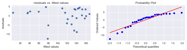
# Linearity and constant variance
pred_val = results.fittedvalues.copy()
true_val = df1.CPI.values.copy()
residual = true_val - pred_val
plt.subplots(figsize = (12, 2.5))
plt.subplot(1, 2, 1)
plt.scatter(pred_val, residual)
plt.xlim([np.min(pred_val) - 2.5, np.max(pred_val) + 2.5])
plt.title("residuals vs. fitted values")
plt.plot(np.mean(residual))
plt.ylabel("residuals")
plt.xlabel("fitted values")
print("Average of residuals: ", np.mean(residual))
# normality of error terms:
plot = plt.subplot(1, 2, 2)
sp.stats.probplot(residual, plot = plot, fit = True)
plt.show()
Average of residuals: -7.868269504775171e-10

model = smf.ols("CPI ~ Year + GDP  + Energy + Tech + Education + Internet + Tourism + Health + C(Country_code)", data = df2)
results = model.fit()
print(results.summary())
                            OLS Regression Results
==============================================================================
Dep. Variable:                    CPI   R-squared:                       0.992
Model:                            OLS   Adj. R-squared:                  0.986
Method:                 Least Squares   F-statistic:                     154.3
Date:                Mon, 03 Jun 2019   Prob (F-statistic):           1.91e-13
Time:                        23:04:03   Log-Likelihood:                -78.305
No. Observations:                  28   AIC:                             182.6
Df Residuals:                      15   BIC:                             199.9
Df Model:                          12
Covariance Type:            nonrobust
=========================================================================================
                            coef    std err          t      P>|t|      [0.025      0.975]
-----------------------------------------------------------------------------------------
Intercept             -6586.6031    858.978     -7.668      0.000   -8417.471   -4755.735
C(Country_code)[T.9]   -145.4794     28.002     -5.195      0.000    -205.165     -85.794
C(Country_code)[T.10]   -70.0538     23.602     -2.968      0.010    -120.360     -19.748
C(Country_code)[T.11]  -280.5317     78.996     -3.551      0.003    -448.909    -112.155
C(Country_code)[T.12]     6.4132     11.911      0.538      0.598     -18.974      31.801
Year                      3.3767      0.445      7.588      0.000       2.428       4.325
GDP                       0.0009      0.001      0.859      0.404      -0.001       0.003
Energy                    0.0019      0.001      2.200      0.044    5.98e-05       0.004
Tech                      6.1411     12.006      0.512      0.616     -19.448      31.731
Education                -1.6565      1.170     -1.416      0.177      -4.150       0.836
Internet                  0.9293      0.175      5.317      0.000       0.557       1.302
Tourism                   0.0003      0.000      1.012      0.327      -0.000       0.001
Health                  -16.6729      6.918     -2.410      0.029     -31.419      -1.927
==============================================================================
Omnibus:                        7.792   Durbin-Watson:                   2.349
Prob(Omnibus):                  0.020   Jarque-Bera (JB):                6.055
Skew:                          -1.071   Prob(JB):                       0.0484
Kurtosis:                       3.774   Cond. No.                     4.12e+07
==============================================================================

Warnings:
[1] Standard Errors assume that the covariance matrix of the errors is correctly specified.
[2] The condition number is large, 4.12e+07. This might indicate that there are
strong multicollinearity or other numerical problems.
# Final MLR model for BRICS:
df2.GDP = df2.GDP ** 0.5
model = smf.ols("CPI ~ Year + GDP + Energy + Internet + Health + C(Country_code)", data = df2)
results = model.fit()
print(results.summary())
                            OLS Regression Results
==============================================================================
Dep. Variable:                    CPI   R-squared:                       0.990
Model:                            OLS   Adj. R-squared:                  0.986
Method:                 Least Squares   F-statistic:                     205.7
Date:                Mon, 03 Jun 2019   Prob (F-statistic):           2.80e-16
Time:                        23:04:03   Log-Likelihood:                -80.832
No. Observations:                  28   AIC:                             181.7
Df Residuals:                      18   BIC:                             195.0
Df Model:                           9
Covariance Type:            nonrobust
=========================================================================================
                            coef    std err          t      P>|t|      [0.025      0.975]
-----------------------------------------------------------------------------------------
Intercept             -6730.8617    734.549     -9.163      0.000   -8274.092   -5187.631
C(Country_code)[T.9]   -128.7403     19.532     -6.591      0.000    -169.775     -87.706
C(Country_code)[T.10]   -59.8789     23.247     -2.576      0.019    -108.718     -11.040
C(Country_code)[T.11]  -215.6060     39.551     -5.451      0.000    -298.699    -132.513
C(Country_code)[T.12]    -3.7484      6.632     -0.565      0.579     -17.682      10.185
Year                      3.4415      0.376      9.164      0.000       2.653       4.230
GDP                       0.2215      0.099      2.242      0.038       0.014       0.429
Energy                    0.0016      0.001      2.742      0.013       0.000       0.003
Internet                  0.9557      0.170      5.623      0.000       0.599       1.313
Health                  -17.8765      6.113     -2.924      0.009     -30.719      -5.034
==============================================================================
Omnibus:                        9.374   Durbin-Watson:                   2.300
Prob(Omnibus):                  0.009   Jarque-Bera (JB):                7.853
Skew:                          -1.232   Prob(JB):                       0.0197
Kurtosis:                       3.814   Cond. No.                     3.30e+07
==============================================================================

Warnings:
[1] Standard Errors assume that the covariance matrix of the errors is correctly specified.
[2] The condition number is large, 3.3e+07. This might indicate that there are
strong multicollinearity or other numerical problems.
# Linearity and constant variance
pred_val = results.fittedvalues.copy()
true_val = df2.CPI.values.copy()
residual = true_val - pred_val
plt.subplots(figsize = (12, 2.5))
plt.subplot(1, 2, 1)
plt.scatter(pred_val, residual)
plt.xlim([np.min(pred_val) - 2.5, np.max(pred_val) + 2.5])
plt.title("residuals vs. fitted values")
plt.plot(np.mean(residual))
plt.ylabel("residuals")
plt.xlabel("fitted values")
print("Average of residuals: ", np.mean(residual))
# normality of error terms:
plot = plt.subplot(1, 2, 2)
sp.stats.probplot(residual, plot = plot, fit = True)
plt.show()
Average of residuals: -3.7022816558516883e-10
model = smf.ols("CPI ~ Year + GDP  + Energy + Tech + Education + Internet + Tourism + Health + C(Group) + C(Country_code)", data = df)
results = model.fit()
print(results.summary())
                            OLS Regression Results
==============================================================================
Dep. Variable:                    CPI   R-squared:                       0.911
Model:                            OLS   Adj. R-squared:                  0.876
Method:                 Least Squares   F-statistic:                     26.34
Date:                Mon, 03 Jun 2019   Prob (F-statistic):           2.11e-19
Time:                        23:04:04   Log-Likelihood:                -249.85
No. Observations:                  69   AIC:                             539.7
Df Residuals:                      49   BIC:                             584.4
Df Model:                          19
Covariance Type:            nonrobust
=========================================================================================
                            coef    std err          t      P>|t|      [0.025      0.975]
-----------------------------------------------------------------------------------------
Intercept             -3231.3455    864.999     -3.736      0.000   -4969.627   -1493.064
C(Group)[T.2]            15.8891     40.173      0.396      0.694     -64.841      96.619
C(Country_code)[T.2]    123.8476     44.646      2.774      0.008      34.129     213.566
C(Country_code)[T.3]    136.6054     46.414      2.943      0.005      43.333     229.878
C(Country_code)[T.4]    119.9816     46.502      2.580      0.013      26.532     213.432
C(Country_code)[T.5]     65.3367     42.810      1.526      0.133     -20.693     151.366
C(Country_code)[T.6]     86.8018     52.690      1.647      0.106     -19.082     192.686
C(Country_code)[T.7]    142.4752     56.167      2.537      0.014      29.604     255.347
C(Country_code)[T.8]     99.5995     20.807      4.787      0.000      57.786     141.413
C(Country_code)[T.9]    -62.9723      8.401     -7.496      0.000     -79.855     -46.090
C(Country_code)[T.10]    48.8000     23.652      2.063      0.044       1.269      96.331
C(Country_code)[T.11]  -159.1432     43.042     -3.697      0.001    -245.640     -72.646
C(Country_code)[T.12]    89.6051     30.215      2.966      0.005      28.886     150.324
Year                      1.6055      0.454      3.537      0.001       0.693       2.518
GDP                      -0.0001      0.000     -0.281      0.780      -0.001       0.001
Energy                    0.0027      0.001      4.868      0.000       0.002       0.004
Tech                     -1.3496      9.336     -0.145      0.886     -20.111      17.412
Education                 2.7756      1.998      1.389      0.171      -1.239       6.790
Internet                  1.2016      0.178      6.749      0.000       0.844       1.559
Tourism               -6.452e-06    9.7e-05     -0.067      0.947      -0.000       0.000
Health                  -13.9396      3.347     -4.165      0.000     -20.665      -7.214
==============================================================================
Omnibus:                        0.080   Durbin-Watson:                   1.641
Prob(Omnibus):                  0.961   Jarque-Bera (JB):                0.210
Skew:                           0.071   Prob(JB):                        0.900
Kurtosis:                       2.771   Cond. No.                     3.28e+17
==============================================================================

Warnings:
[1] Standard Errors assume that the covariance matrix of the errors is correctly specified.
[2] The smallest eigenvalue is 3.58e-24. This might indicate that there are
strong multicollinearity problems or that the design matrix is singular.
# transformation on GDP for BRICS:
df.GDP = df.GDP ** 0.5
simplified = smf.ols("CPI ~ Year + GDP + C(Group) + C(Country_code) + Tech + Internet + Health + Energy", data = df)
results = simplified.fit()
print(results.summary())
                            OLS Regression Results
==============================================================================
Dep. Variable:                    CPI   R-squared:                       0.910
Model:                            OLS   Adj. R-squared:                  0.880
Method:                 Least Squares   F-statistic:                     30.27
Date:                Mon, 03 Jun 2019   Prob (F-statistic):           9.00e-21
Time:                        23:04:04   Log-Likelihood:                -250.23
No. Observations:                  69   AIC:                             536.5
Df Residuals:                      51   BIC:                             576.7
Df Model:                          17
Covariance Type:            nonrobust
=========================================================================================
                            coef    std err          t      P>|t|      [0.025      0.975]
-----------------------------------------------------------------------------------------
Intercept             -2503.6766    831.666     -3.010      0.004   -4173.316    -834.037
C(Group)[T.2]            28.2617     37.919      0.745      0.459     -47.863     104.386
C(Country_code)[T.2]    116.2253     42.636      2.726      0.009      30.631     201.820
C(Country_code)[T.3]    127.9353     43.953      2.911      0.005      39.697     216.174
C(Country_code)[T.4]    107.7949     44.611      2.416      0.019      18.235     197.355
C(Country_code)[T.5]     59.8152     41.060      1.457      0.151     -22.616     142.247
C(Country_code)[T.6]     83.3700     48.743      1.710      0.093     -14.486     181.226
C(Country_code)[T.7]    130.6017     52.881      2.470      0.017      24.440     236.764
C(Country_code)[T.8]    108.8645     17.731      6.140      0.000      73.268     144.461
C(Country_code)[T.9]    -62.3304      8.314     -7.497      0.000     -79.020     -45.640
C(Country_code)[T.10]    55.8243     21.267      2.625      0.011      13.128      98.520
C(Country_code)[T.11]  -187.6129     28.547     -6.572      0.000    -244.924    -130.302
C(Country_code)[T.12]   113.5162     20.805      5.456      0.000      71.748     155.284
Year                      1.2482      0.439      2.843      0.006       0.367       2.130
GDP                       0.1542      0.123      1.254      0.216      -0.093       0.401
Tech                     -2.6374      8.980     -0.294      0.770     -20.666      15.391
Internet                  1.2893      0.161      8.032      0.000       0.967       1.612
Health                  -14.8170      2.943     -5.035      0.000     -20.725      -8.909
Energy                    0.0027      0.001      5.369      0.000       0.002       0.004
==============================================================================
Omnibus:                        0.717   Durbin-Watson:                   1.451
Prob(Omnibus):                  0.699   Jarque-Bera (JB):                0.253
Skew:                           0.091   Prob(JB):                        0.881
Kurtosis:                       3.235   Cond. No.                     4.22e+18
==============================================================================

Warnings:
[1] Standard Errors assume that the covariance matrix of the errors is correctly specified.
[2] The smallest eigenvalue is 5.5e-27. This might indicate that there are
strong multicollinearity problems or that the design matrix is singular.
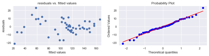
Checking assumptions of linear model:
# Linearity and constant variance
pred_val = results.fittedvalues.copy()
true_val = df.CPI.values.copy()
residual = true_val - pred_val
plt.subplots(figsize = (12, 2.5))
plt.subplot(1, 2, 1)
plt.scatter(pred_val, residual)
plt.xlim([np.min(pred_val) - 2.5, np.max(pred_val) + 2.5])
plt.title("residuals vs. fitted values")
plt.plot(np.mean(residual))
plt.ylabel("residuals")
plt.xlabel("fitted values")
print("Average of residuals: ", np.mean(residual))
# normality of error terms:
plot = plt.subplot(1, 2, 2)
sp.stats.probplot(residual, plot = plot, fit = True)
plt.show()
Average of residuals: 2.441826451183221e-11

Modeling on other countries from G20 (not in G7 nor in BRICS):
# testing on G20 countries (not in G7 nor in BRICS) (Note: no data entry for South Korea, and only one entry for Argentina)
# added test countries: New Zealand and Singapore
testing = ["Australia", 'Saudi Arabia', 'India', 'Turkey', 'Mexico', 'Indonesia', 'New Zealand', 'Singapore']  # Argentina
CPI.loc[years, testing]
| Country | Australia | Saudi Arabia | India | Turkey | Mexico | Indonesia | New Zealand | Singapore |
|---|---|---|---|---|---|---|---|---|
| Year | ||||||||
| 1995 | 67.6 | NaN | 37.6 | 1.3 | 26.4 | 19.4 | 71.7 | 81.5 |
| 2005 | 86.3 | 81.4 | 65.8 | 65.9 | 80.5 | 68.7 | 87.0 | 88.0 |
| 2014 | 110.4 | 112.9 | 140.8 | 135.7 | 116.2 | 124.4 | 107.6 | 113.8 |
| 2015 | 112.0 | 114.4 | 147.7 | 146.1 | 119.4 | 132.3 | 107.9 | 113.2 |
| 2016 | 113.5 | 116.7 | 155.0 | 157.4 | 122.8 | 137.0 | 108.6 | 112.6 |
| 2017 | 115.7 | 115.7 | 160.1 | 175.0 | 130.2 | 142.2 | 110.7 | 113.3 |
df_test = pd.DataFrame()
for name in testing:
    table = pd.DataFrame(CPI.stack().loc[list(years), name])
    table = pd.concat([table, pd.DataFrame(GDP.stack().loc[list(years), name]), pd.DataFrame(energy.stack().loc[list(years), name]), pd.DataFrame(tech.stack().loc[list(years), name]), pd.DataFrame(education.stack().loc[list(years), name]), pd.DataFrame(rates.stack().loc[list(years), name]), pd.DataFrame(internet.stack().loc[list(years), name]), pd.DataFrame(tourism.stack().loc[list(years), name]), pd.DataFrame(health.stack().loc[list(years), name])], keys = ["CPI", "GDP", "Energy", "Tech", "Education", "Rates", "Internet", "Tourism", "Health"], axis = 1)
    table.fillna(method = "ffill", inplace = True)
    table.fillna(method = "bfill", inplace = True)
    df_test = pd.concat([df_test, table])

df_test.fillna(0, inplace = True)

df_test.columns = df_test.columns.droplevel(1)
df_test["Country"] = df_test.index.get_level_values(1)
df_test.index = df_test.index.droplevel(1)
df_test.reset_index(inplace = True)
code_test = {"Australia" : 13, "Saudi Arabia" : 14, "India" : 15, "Turkey" : 16, "Mexico" : 17, "Indonesia" : 18, 'New Zealand' : 19, 'Singapore' : 20}
group_code = {"Australia" : 1, "Saudi Arabia" : 1, "India" : 2, "Turkey" : 2, "Mexico" : 2, "Indonesia" : 2, 'New Zealand' : 1, 'Singapore' : 1}

df_test["Country_code"] = [code_test[country] for country in df_test.Country]
df_test["Group"] = [group_code[country] for country in df_test.Country]
df_test.head()
| Year | CPI | GDP | Energy | Tech | Education | Rates | Internet | Tourism | Health | Country | Country_code | Group | |
|---|---|---|---|---|---|---|---|---|---|---|---|---|---|
| 0 | 1995 | 67.6 | 21635.0 | 7784.0 | 1.9 | 13.6 | 1.3 | 63.0 | 10370.0 | 8.0 | Australia | 13 | 1 |
| 1 | 2005 | 86.3 | 37571.0 | 11451.0 | 1.9 | 13.6 | 1.3 | 63.0 | 19719.0 | 8.0 | Australia | 13 | 1 |
| 2 | 2014 | 110.4 | 37571.0 | 15272.0 | 1.9 | 13.9 | 1.1 | 84.0 | 19719.0 | 9.1 | Australia | 13 | 1 |
| 3 | 2015 | 112.0 | 52388.0 | 15930.0 | 1.9 | 13.9 | 1.3 | 84.6 | 30872.0 | 9.4 | Australia | 13 | 1 |
| 4 | 2016 | 113.5 | 54067.0 | 16322.0 | 1.9 | 13.9 | 1.3 | 86.5 | 36786.0 | 9.4 | Australia | 13 | 1 |
x_test = df_test.iloc[:, [0,2,3,4,5,6,7,8,9,11,12]]
y_test = df_test.iloc[:, 1]

x_test.reset_index(inplace = True)
x = pd.concat([x_test, pd.DataFrame(encode.fit_transform(x_test[["Group"]]), columns = ["G7", "BRICS"])], axis = 1)
x.drop("index", axis = 1, inplace = True)

# for MLR modeling:
df_testing = pd.concat([x, y_test.reset_index().iloc[:, 1]], axis = 1)
x.head()
| Year | GDP | Energy | Tech | Education | Rates | Internet | Tourism | Health | Country_code | Group | G7 | BRICS | |
|---|---|---|---|---|---|---|---|---|---|---|---|---|---|
| 0 | 1995 | 21635.0 | 7784.0 | 1.9 | 13.6 | 1.3 | 63.0 | 10370.0 | 8.0 | 13 | 1 | 1.0 | 0.0 |
| 1 | 2005 | 37571.0 | 11451.0 | 1.9 | 13.6 | 1.3 | 63.0 | 19719.0 | 8.0 | 13 | 1 | 1.0 | 0.0 |
| 2 | 2014 | 37571.0 | 15272.0 | 1.9 | 13.9 | 1.1 | 84.0 | 19719.0 | 9.1 | 13 | 1 | 1.0 | 0.0 |
| 3 | 2015 | 52388.0 | 15930.0 | 1.9 | 13.9 | 1.3 | 84.6 | 30872.0 | 9.4 | 13 | 1 | 1.0 | 0.0 |
| 4 | 2016 | 54067.0 | 16322.0 | 1.9 | 13.9 | 1.3 | 86.5 | 36786.0 | 9.4 | 13 | 1 | 1.0 | 0.0 |
# new model for new observations:
model = smf.ols("CPI ~ Year + GDP  + Energy + Tech + Education + Internet + Tourism + Health + C(Group) + C(Country_code)", data = df_testing)
results = model.fit()
print(results.summary())
                            OLS Regression Results
==============================================================================
Dep. Variable:                    CPI   R-squared:                       0.948
Model:                            OLS   Adj. R-squared:                  0.924
Method:                 Least Squares   F-statistic:                     38.88
Date:                Mon, 03 Jun 2019   Prob (F-statistic):           2.84e-16
Time:                        23:04:06   Log-Likelihood:                -169.72
No. Observations:                  48   AIC:                             371.4
Df Residuals:                      32   BIC:                             401.4
Df Model:                          15
Covariance Type:            nonrobust
=========================================================================================
                            coef    std err          t      P>|t|      [0.025      0.975]
-----------------------------------------------------------------------------------------
Intercept             -6069.9806   1058.992     -5.732      0.000   -8227.077   -3912.884
C(Group)[T.2]          -115.3155     35.407     -3.257      0.003    -187.437     -43.194
C(Country_code)[T.14]  -193.1812     59.377     -3.253      0.003    -314.129     -72.233
C(Country_code)[T.15]   -23.6169     18.441     -1.281      0.210     -61.180      13.946
C(Country_code)[T.16]    -0.2754     12.239     -0.023      0.982     -25.205      24.654
C(Country_code)[T.17]    -6.1609     17.699     -0.348      0.730     -42.214      29.892
C(Country_code)[T.18]   -85.2623     25.712     -3.316      0.002    -137.636     -32.889
C(Country_code)[T.19]    -0.3094     34.249     -0.009      0.993     -70.072      69.453
C(Country_code)[T.20]  -158.1443     33.346     -4.743      0.000    -226.067     -90.221
Year                      3.1666      0.528      5.999      0.000       2.091       4.242
GDP                      -0.0004      0.000     -0.758      0.454      -0.001       0.001
Energy                    0.0019      0.001      1.543      0.133      -0.001       0.004
Tech                    -17.1896     26.899     -0.639      0.527     -71.982      37.602
Education                 3.8034      1.975      1.926      0.063      -0.220       7.827
Internet                  0.9502      0.240      3.965      0.000       0.462       1.438
Tourism                   0.0004      0.000      0.798      0.431      -0.001       0.001
Health                  -34.8388      5.737     -6.073      0.000     -46.524     -23.153
==============================================================================
Omnibus:                        0.936   Durbin-Watson:                   2.523
Prob(Omnibus):                  0.626   Jarque-Bera (JB):                0.290
Skew:                          -0.062   Prob(JB):                        0.865
Kurtosis:                       3.360   Cond. No.                     7.61e+17
==============================================================================

Warnings:
[1] Standard Errors assume that the covariance matrix of the errors is correctly specified.
[2] The smallest eigenvalue is 8.07e-26. This might indicate that there are
strong multicollinearity problems or that the design matrix is singular.
df_testing.GDP = df_testing.GDP ** 0.5
# new model for new observations:
model = smf.ols("CPI ~ Year + GDP  + Energy + Internet + Health + Education + C(Group) + C(Country_code)", data = df_testing)
results = model.fit()
print(results.summary())
                            OLS Regression Results
==============================================================================
Dep. Variable:                    CPI   R-squared:                       0.946
Model:                            OLS   Adj. R-squared:                  0.925
Method:                 Least Squares   F-statistic:                     45.39
Date:                Mon, 03 Jun 2019   Prob (F-statistic):           1.29e-17
Time:                        23:04:06   Log-Likelihood:                -170.83
No. Observations:                  48   AIC:                             369.7
Df Residuals:                      34   BIC:                             395.9
Df Model:                          13
Covariance Type:            nonrobust
=========================================================================================
                            coef    std err          t      P>|t|      [0.025      0.975]
-----------------------------------------------------------------------------------------
Intercept             -6002.8626   1074.099     -5.589      0.000   -8185.695   -3820.030
C(Group)[T.2]           -97.8380     16.180     -6.047      0.000    -130.719     -64.957
C(Country_code)[T.14]  -172.2523     19.629     -8.775      0.000    -212.144    -132.361
C(Country_code)[T.15]   -33.3714     17.276     -1.932      0.062     -68.481       1.738
C(Country_code)[T.16]     9.1391      9.694      0.943      0.352     -10.560      28.839
C(Country_code)[T.17]     5.0922     13.325      0.382      0.705     -21.987      32.171
C(Country_code)[T.18]   -78.6978      9.685     -8.126      0.000     -98.380     -59.016
C(Country_code)[T.19]    17.9422     22.280      0.805      0.426     -27.337      63.221
C(Country_code)[T.20]  -161.9414     27.432     -5.903      0.000    -217.690    -106.193
Year                      3.1247      0.542      5.760      0.000       2.022       4.227
GDP                      -0.0769      0.124     -0.619      0.540      -0.329       0.176
Energy                    0.0026      0.001      2.399      0.022       0.000       0.005
Internet                  0.9800      0.188      5.199      0.000       0.597       1.363
Health                  -36.1075      4.130     -8.742      0.000     -44.501     -27.714
Education                 3.3403      1.883      1.774      0.085      -0.486       7.167
==============================================================================
Omnibus:                        0.915   Durbin-Watson:                   2.531
Prob(Omnibus):                  0.633   Jarque-Bera (JB):                0.270
Skew:                          -0.002   Prob(JB):                        0.874
Kurtosis:                       3.367   Cond. No.                     3.32e+17
==============================================================================

Warnings:
[1] Standard Errors assume that the covariance matrix of the errors is correctly specified.
[2] The smallest eigenvalue is 9.06e-26. This might indicate that there are
strong multicollinearity problems or that the design matrix is singular.
# Linearity and constant variance
pred_val = results.fittedvalues.copy()
true_val = df_testing.CPI.values.copy()
residual = true_val - pred_val
plt.subplots(figsize = (12, 2.5))
plt.subplot(1, 2, 1)
plt.scatter(pred_val, residual)
plt.xlim([np.min(pred_val) - 2.5, np.max(pred_val) + 2.5])
plt.title("residuals vs. fitted values")
plt.plot(np.mean(residual))
plt.ylabel("residuals")
plt.xlabel("fitted values")
print("Average of residuals: ", np.mean(residual))
# normality of error terms:
plot = plt.subplot(1, 2, 2)
sp.stats.probplot(residual, plot = plot, fit = True)
plt.show()
Average of residuals: -9.378579394573687e-11
6. Results and Analysis:
Part I: predicting CPI range (categorical)
Results:
- G7 countries:
- KNN: tends to predict higher CPI range.
- Naive Bayes: tends to predict higher CPI range.
- Summary: two classifiers have very similar classification outcomes.
- BRICS:
- KNN: tends to predict higher CPI range.
- Naive Bayes: correctly classified all labels in the testing set.
- Summary: has higer correct classification rate than KNN.
- G7 and BRICS:
- KNN: tends to have misclassifications on class 1 and class 3.
- Naive Bayes: tends to have misclssifications on class 1.
- Summary: Naive Bayes classifier classifies the label better than KNN classifier.
Analysis:
(1) Analysis on two types of classifiers:
- In KNN classifier, we are looking for the neareast neighbors based on Euclidean distances to decide which class the input belongs to.
- In Naive Bayes classifier, we assumed that predictor variables are independent from each other. This is an important simpification in our model, since the macroeconomic predictors (such as GDP, expenditure on energy, expenditure on education, etc.) that we have choosen to use are, to some degree, independent factors that represent the economic growth of countries.
- Based on the fact that Naive Bayes classifier has a reasonable assumption that can largely simplify the analysis and increase the accuracy of the classification, we suggest using Naive Bayes classification method in this model.
(2) Analysis on three ways of making the classification:
- In the classification for G7 countries, it can be observed that there are only two possible labels for the range of CPI: 1 (low CPI) and 2 (moderate CPI).
- In the classification for BRICS countries, there are four different labels for the range of CPI, varying from 1 to 4.
- The difference between the total number of output classes reflects the fact that these two groups of countries have quite different economic growth pattern, i.e., the developed countries in G7 tend to have more stable range of CPI, while the developing countries in BRICS tend to have more fluctuations in the range of CPI.
- This difference between CPI of G7 and BRICS can be observed from the output of three classifications: the correct classification rate is higher when we seperated countries into G7 and BRICS countries.
- Therefore, it is more reasonable to analyze the CPI range of G7 and BRICS countries seperately, based on the situation that developed countries and developing countries tend to have large amount of variation in their ecnomic growth pattern.
Part II: predicting CPI value (numeric)
Results:
- MLR model for G7 countries:
- $R^{2}_{adj}$: 0.906
- CV score: 0.6131
- BRICS:
- $R^{2}_{adj}$: 0.986
- CV score: 0.6869
- G7 and BRICS:
- $R^{2}_{adj}$: 0.870
- CV score: 0.8208
- New testing set of countries:
- $R^{2}$: 0.2678
- $R^{2}_{adj}$ of new model: 0.924
Analysis:
ANOVA:
Based on the ANOVA for each three types of models - G7, BRICS, and two groups combined, we notice that the multiple linear regression models for G7 and BRICS both have very high $R^{2}_{adj}$, meaning that the variables selected can explain a large amount of variation of CPI.
(1) From ANOVA of G7, it can be observed that variables Tech, Education, Tourism, Internet and Rates are not statistically significant predictors, based on significance level $\alpha = 0.05$. After removing these five predictors from the model, we notice that our model is highly simplified, and at the same token, the $R^{2}_{adj}$ of the model remains at 0.947.
Thus, our final model for G7 countries is:
(2) From ANOVA of BRICS, we observe that predictors GDP, Tech, Education and Tourism are not statistically significant in predicting the response, using significance level $\alpha = 0.05$. Instead of removing all of these insignificant predictors, we decided to make a transformation on GDP, and remove the other three predictors. After performing the transformation on GDP and removing three predictors, we observe that the $R^{2}_{adj}$ of the new reduced model remains at 0.986.
Thus, our final model for BRICS countries is:
(3) Similarly, from the ANOVA for two groups combined, we observe that GDP, Tech, Education and Tourism are not statistically significant predictors. After transforming GDP and removing other predictors, we see that $R^{2}_{adj}$ actually increased to be 0.880.
Therefore, the final model for two groups combined is:
Cross Validation:
Although $R^{2}_{adj}$ of regression models on G7 and on BRICS are both above 90%, when we did cross validation on these two models, the cv scores are not as good as the cv score for regression model using G7 and BRICS combined. This shows that when we seperate our data into G7 and BRICS and build two models, the model tends to be overfitting (low bias but high variance); similarly, when we build a model for two groups of countries combined, the model also tends to be overfitting (low bias but high variance).
MLR model on new observations:
In addition to cross validating the models, we also took a look at how would the model be like when there are new observations. We selected some countries from G20 that are not inside G7 and not inside BRICS, and a few more countries. The new set of observations consists of both developed countries and developing countries, which is similar to what we have in the model for G7 and BRICS combined. The new observations that we selected are Australia, Saudi Arabia, India, Turkey, Mexico, Indonesia, New Zealand, and Singapore.
Based on the ANOVA output of two different models, the full model and the reduced model, we observe that the reduced model employs fewer predictors, but has a higher $R^{2}_{adj}$ score.
Similar to what we have in the G7 and BRICS combined model, the MLR model we decided to use for the new observations is:
7. Conclusion and Discussion:
Classification designs:
- KNN classifier and Naive Bayes classifier have very similar classification performances.
- However, Naive Bayes classifier, in general, has a higher classification correction rate.
- The important assumption in Naive Bayes is that predictor variables are independent. This is a reasonable assumption in our modeling, since the predictor variables are macro-economics variables that can be seen approximately independent from each other.
- Based on this assumption of Naive Bayes classifier, which highly simpifies the classification model and maintains a good performance, we suggest using this classifier in predicting the range of CPI.
Regression designs:
- In MLR models for G7 and BRICS, it can be observed that important predictor variables for both models are Year, GDP, Energy, Health and country name itself.
- In MLR model for G7 and BRICS combined, it can be easily seen that Year, GDP, Energy, Health, country name and group category are important predictors.
- The fact that group code is a statistically significant predictor variable shows countries in G7 (mostly highly developed ones) and countries in BRICS (developing countries with rapid economic growth) have quite different economic growth pattern. This difference in these two groups suggest that it might be a better idea to model CPI of developed countries and developing separately.
- However, the drawback of building two indiviual models is overfitting issue. It can be clearly seen that models for G7 and BRICS have a relatively higher $R^{2}_{adj}$ than that in the model for two groups combined. But based on cross validation, we see that the variance of the error of prediction in these two models is quite large.
- Therefore, our suggestion is we should choose which model to use based on the context: if we want to predict CPI for only developed countries (or developing countries), it would be better to build a model using training data of developed countries (or developing countries) only; on the other hand, if we want a general model for predictin CPI for both developed countries and developing ones, it would be optimal to build the model based on training data containing both types of countries.
Discussion and possible improvements:
- Since we only chose to predict CPI for countries from G7 and BRICS, the size of the training data is not very large. We would like to incorporate more entries of other countries into our modeling to enhance the model performance.
- We also want to further explore the between the devlopment difference between G7 and BRICS countries. Although CPI is not calculated based on hard metrics (it is a reflection of the fluctuation of prices), it would be interesting to see how CPI is related to certain variables at macroeconomic level.